Discrete Probability Distributions: Overview (Series)

In my previous two posts I sketched the frame of the big picture around probability distributions. In my introductory post I gave some intuition about the general concept and talked about the two major kinds: discrete and continuous distributions. And in the follow-up post I related the concepts of mean and variance to probability distributions. I showed that this connection itself goes through two fundamental concepts from probability theory: the law of large numbers and expected value.

Now I want to build on all these posts. My plan is to start introducing commonly used discrete and continuous distributions in separate posts dedicated to each one. And I want to start with the former, since they are significantly easier to understand.

The goal of the current post is to be a final warm-up before delving into the details of specific distributions.

I’m going to give an overview of discrete probability distributions in general. Namely, I want to talk about a few other basic concepts and terminology around them and briefly introduce the 6 most commonly encountered distributions (as well as a bonus distribution):

• Bernoulli distribution
• binomial distribution
• categorical distribution
• uniform distribution
• geometric distribution
• Poisson distribution
• Skellam distribution (bonus)

For now I’m going to give an overview of these distributions. But as I add the dedicated posts to this series, I’m going to move most of the information there (with a lot more details). The titles above are going to become active links one by one, as I publish the posts dedicated to each distribution.

If you’re not too familiar with probability distributions, I would recommend reading the 2 related posts I linked above before continuing.

The sample space of a discrete random variable

If you’ve been following my posts, you should already have a good familiarity with sample spaces. A sample space is simply the set of all possible outcomes of a random variable.

The sample space of a discrete random variable consists of distinct elements. Unlike continuous random variables, whose domain is the set of real numbers, here there are “gaps” between the elements. Meaning, there aren’t infinitely many values between any pair of elements.

However, even discrete random variables can have a sample space with an infinite number of elements (while still having gaps between them). How can that be?

Finite versus infinite discrete sample spaces

Let’s look at a few examples of discrete sample spaces:

• Flipping a coin: {Heads, Tails}
• Rolling a die: {1, 2, 3, 4, 5, 6}
• The sex of a randomly picked animal from a forest: {Male, Female}
• The number of “heads” out of 4 consecutive coin flips: {0, 1, 2, 3, 4}
• Whether the winner of this season’s Champions League will be an English team: {Yes, No}

All of these are finite in size. But even discrete sample spaces can have an infinite number of elements. For example:

• The number of “tails” before the first “heads” appears in a sequence of coin flips: {0, 1, 2, 3, 4, 5, 6, …, ∞}
• The number of cars that pass through some intersection during a particular 24-hour period: {0, 1, 2, 3, 4, 5, 6, …, ∞}

Why are these infinite?

Well, take the first example. Even with a fair coin, it’s possible to flip 10 “tails” in a row, right? It’s also possible to flip 100 “tails” in a row. Technically, it’s possible to flip an arbitrary number of “tails” before the first “heads” appears (even though the probabilities decrease exponentially for each additional “tails”). And since the definition of a sample space is “the set of all possible outcomes”, this one has an infinite number of elements.

The second example is a bit trickier. You might object that there are physical limits to the number of cars that can pass through an intersection over any period of time. And you’d be right, this is a somewhat idealized example. Namely, it has the idealistic assumption that there are infinitely many cars and it takes an infinitesimal instance for one car to pass through the intersection. I’ll come back to this in the section about Poisson distributions below.

Discrete sample spaces and natural numbers

As you can see in the examples above, the elements of a discrete sample space can be of any kind. Sometimes they’re numbers, sometimes they’re logical truth values (“yes”/”no”), sometimes they’re biological sexes of animals, and so on.

But can we find a way to represent all discrete sample spaces in the same terms? To help you get a better intuition about them, I’m going to do just that.

What if I told you that you can represent the sample space of any discrete random variable as a subset of the set of natural numbers?

The set of natural numbers

If you’d like to get a deeper intuition about natural numbers and real numbers in general, check out my series on numbers and arithmetic.

The set of natural numbers consists of all non-negative whole numbers (0, 1, 2, 3, 4, … all the way to infinity). Not only is this set infinite, but it is actually the “smallest” possible infinite set that exists.

Natural numbers are a subset of real numbers. This means that every natural number is also a real number. Other subsets of real numbers include:

• integers: all natural numbers and their negatives
• rational numbers: all ratios of integers
• algebraic numbers: all numbers which are solutions to polynomial equations with integer coefficients

To give some intuition about these sets, I’m going to borrow two images from this awesome article that introduces real (and complex) numbers and their various subsets.

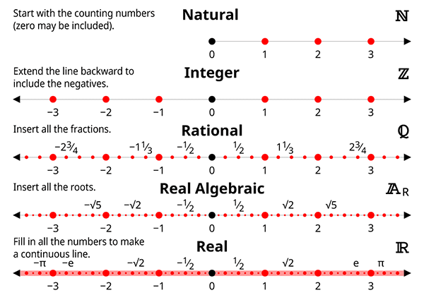
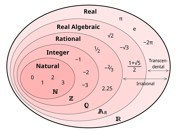
I just said that natural numbers are the smallest possible infinite set. What does that mean? Well, it means that any other infinite set’s size is greater than or equal to that of the natural numbers. For example, the sets of integers and rational numbers have the same size as natural numbers. On the other hand, the set of real numbers is larger than all three. How can that be?

You may have 2 possible objections here:

1. Don’t all infinite sets have the same size? After all, they are infinite!
2. Aren’t integers more than natural numbers? After all, all natural numbers are integers but not all integers are natural numbers!

Well, the answer to both questions is ‘no’.

First, there are many types of infinities. In fact, there are an infinite number of infinities! This is a complicated topic and I won’t go into much detail here. If you’re curious to learn more, check out this Wikipedia article.

I’m going to focus a bit more on the second question in the next section.

Mapping a discrete sample space to natural numbers

To map a set to another set simply means to associate the elements of the first set to the elements of the second through a function (I defined functions in the introductory post on probability distributions and more comprehensively in the post dedicated to functions).

Well, the sample space is a set, so it can also be mapped to other sets.

Let’s look at a few examples:

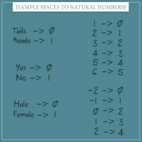
Here we map the elements of a discrete sample space to the first N natural numbers (where N is the size of the respective sample space). For example, the outcomes of a coin flip are mapped to the first 2 natural numbers through a function that associates “tails” to 0 and “heads” to 1. Similarly, the outcomes of a die roll (top right) are mapped to the first 6 natural numbers.

You might not immediately see the point of this exercise, but stay with me.

Mapping finite sample spaces seems easy enough. But what about infinite sample spaces?

Let’s take a random variable whose sample space is the set of all integers (if you want to see an example of an actual distribution with such a sample space, take a look at the Skellam distribution I define below). Remember earlier I said that integers and natural numbers have the same size? Well, now you’re going to see why.

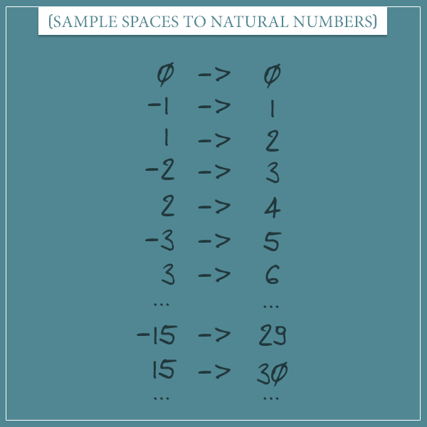
On the right you see all natural numbers in order. And on the left you see the set of integers. The rule to associate an integer to a natural number is the following:

1. If the integer is positive or zero, multiply it by 2.
2. If the integer is negative, take its absolute value, multiply it by 2, and subtract 1 from the product.

In other words, map non-negative integers to even natural numbers and negative integers to odd natural numbers.

Countable versus uncountable infinities

With the last example above, we reach an important topic in set theory. A set is said to be countable if you can find a one-to-one function from it to a subset of the natural numbers.

Intuitively, this means that you can actually enumerate the elements of the set in some specific order (you can “count” them).

A set is said to be countably infinite if you can find a one-to-one function that maps its elements to the full set of natural numbers. This is exactly what we did in the last example. In other words, the set of integers is countably infinite, because we were able to construct a one-to-one function from it to the set of natural numbers.

Perhaps now you understand better why integers and natural numbers have the same size. You see, there is a one-to-one correspondence between their elements. This allows you to define things like “the first integer”, “the fifth integer”, “the millionth integer”, and so on. Just like you can “naturally” do with natural numbers.

You might be wondering if we can’t use a similar trick and map the whole set of real numbers to the set of natural numbers. Well, the answer is ‘no’. The great 19th century mathematician Georg Cantor (who founded modern set theory) proved that it’s impossible to construct a one-to-one function from real numbers to natural numbers. Even though the proof itself isn’t difficult to follow, I’m not going to diverge too much in this post. However, if you’re curious, you can check out the Wikipedia article on Cantor’s proof.

The fact that real numbers can’t be mapped to natural numbers in a one-to-one manner gives birth to the concept of uncountable sets. Unlike integers and rational numbers, the set of real numbers is uncountably infinite.

Why map discrete sample spaces to natural numbers?

So, after all, what was the point of showing how sample spaces of discrete probability distributions can be mapped to natural numbers?

Well, I mostly wanted to give you intuition about what it means for a sample space to be discrete. We already know that the domain of continuous sample spaces is the set of real numbers. If it were possible to map the real numbers to natural numbers with a one-to-one function, the distinction between discrete and continuous sample spaces would be quite blurred (in fact, it would probably be nonexistent).

But now we have a very precise demarcation between the two classes of sample spaces (and, hence, the two classes of probability distributions). Namely, a discrete sample space is one whose size (number of elements) is less than or equal to the set of natural numbers.

I want to emphasize that you don’t really have to do this mapping when working with discrete probability distributions. When dealing with specific random variables, you typically work directly in their natural domain ({Heads, Tails}, {Male, Female}, etc.). But I think putting all discrete sample spaces in the same terms helps in comparing different distributions. That is why I’m going to focus on sample spaces whose elements are natural numbers when introducing specific distributions below.

Well, after this long discussion on sample spaces, let’s get to another important topic related to discrete probability distributions. After that, I am finally going to show a few specific distributions frequently encountered in probability theory.

Parameters of a discrete probability distribution

As you already know, a discrete probability distribution is specified by a probability mass function. This function maps every element of a random variable’s sample space to a real number in the interval [0, 1]. Namely, to the probability of the corresponding outcome.

The probability mass function has two kinds of inputs. The first is the outcome whose probability the function will return. The second is the parameters of the probability distribution.

A parameter is a value that, roughly speaking, modifies the “shape” of the distribution. Parameters change the behavior of a probability distribution which leads to the same outcomes getting different probabilities. In other words, the parameters modify the probabilities assigned to the outcomes of a random variable. This is still a bit abstract, but you’ll see examples of how this works for specific distributions in a bit.

A common notation for writing probability mass functions is to put the outcome as the first input. Then you list all of its parameters, separated from the outcome by a semicolon:

Here, “outcome” stands for an arbitrary element of the sample space. And p1, p2, … stand for the first parameter, the second parameter, and so on.

A more compact way of expressing a probability mass function is:

   

This represents a probability distribution with two parameters, called m and n. The x stands for an arbitrary outcome of the random variable.

With all this background information in mind, let’s finally take a look at some real examples of discrete probability distributions.

Commonly used discrete probability distributions

I’m going to split this section in two parts.

In the first part, I’m going to introduce the following discrete probability distributions with finite sample spaces:

• Bernoulli distribution
• Binomial distribution
• Categorical distribution
• Uniform distribution

And, in the second part, I’m going to introduce 3 distributions with infinite sample spaces:

• Geometric distribution
• Poisson distribution
• Skellam distribution

I want to relate each distribution to some real world process. And to allow better comparison between distributions, I’m going to use the same kind of example for each of them. Namely, the process of randomly drawing a ball from a large pool of balls of different colors.

Each kind of general distribution is actually a class of specific distributions. That is, there is infinitely many distributions of each kind, determined by the value of their parameters.

Discrete distributions with a finite sample space

The Bernoulli distribution

Say you have a large pool of balls, of which some percentage are green and the rest are red. If you randomly draw one ball, what is the probability that it will be green?

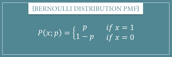
The answer to this question is given by a Bernoulli distribution. This is a distribution with a single parameter, often called p (a real number between 0 and 1) which represents the probability of one of the outcomes.

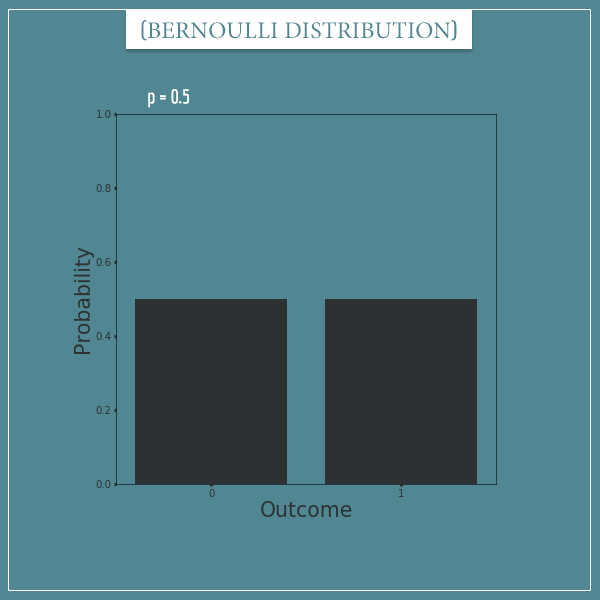
If the percentage of green balls is 50% and we decide to label trials in which a green ball is drawn “success” trials, then drawing a single ball would be governed by a Bernoulli distribution with a parameter p = 0.5. If the percentage is 25%, p would be 0.25. You get the idea. This is what a Bernoulli distribution with p = 0.5 looks like:

And here’s what the probability mass function of a Bernoulli distribution looks like:

Curious about the details? Check out my post dedicated to the Bernoulli distribution.

The binomial distribution

Let’s continue with the same example to introduce another celebrity among discrete probability distributions.

Say you have a pool of red and green balls. You draw a ball at random and then throw it back inside the pool and mix the balls. If you repeat this 5 times, what is the probability that you will draw exactly 3 green balls?

To answer such questions, we need a binomial distribution. More generally, a binomial distribution is about the probability of getting x successes out of n independent trials, where each trial has a Bernoulli distribution with the same parameter p.

Therefore, a binomial distribution has 2 parameters: p and n. Here p is the parameter of the Bernoulli distribution that defines each independent trial and n is the number of trials. In a way, the Bernoulli distribution is a special case of the binomial distribution. That is, a Bernoulli distribution is simply a binomial distribution with the parameter n equal to 1.

This is the probability mass function of a binomial distribution:

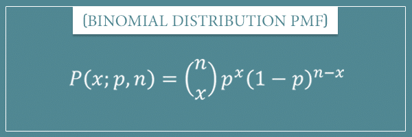
The first term is the binomial coefficient I introduced in my post about combinatorics:

   

Namely, the number of ways in which you can arrange x objects into n slots.

For example, let’s take a binomial distribution with p = 0.3 and n = 3. That is, we have a pool of 30% green balls and 70% red balls and we’re drawing 3 balls at random. Let’s say we want to calculate the probability of exactly 2 of them being green:

   

   

   

Pretty simple, isn’t it?

Here’s a plot of a binomial distribution with parameters p = 0.5 and n = 5:

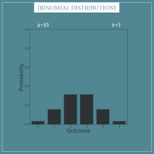
Curious about the details? Check out my post dedicated to the binomial distribution.

The categorical distribution

Now let’s say you have a pool of red, green, blue, and black balls. And the percentages are:

• Red: 30%
• Green: 20%
• Blue: 10%
• Black: 40%

If you draw a single ball, what is the probability of it being of a particular color?

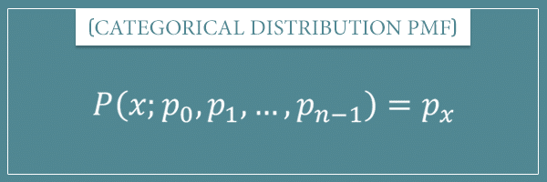
This probability is given by a categorical distribution. The categorical distribution describes random variables which have an arbitrary number of possible outcomes. This distribution has n parameters, where n is the number of possible outcomes. If we label the outcomes with the first n integers, then the parameters could be labeled p₀, p₁, p₂, … p_n-1.

Notice that, unlike the previous two distributions, the categorical distribution has a variable number of parameters!

The probability mass function simply associates each outcome to its corresponding parameter:

Earlier I said that the binomial distribution is a generalization of the Bernoulli distribution. Well, the categorical distribution is also a generalization of the Bernoulli distribution, but in a different direction.

The Bernoulli distribution is a special case of the binomial distribution where the parameter n is fixed to 1. Similarly, it is a special case of the categorical distribution where the number of possible outcomes is fixed to only 2.

In case you’re wondering, there is also a generalization which allows both more than 2 outcomes and more than 1 trial. This is the multinomial distribution. The multinomial distribution is also encountered very frequently in a wide variety of domains, but I am going to leave its introduction for a future post.

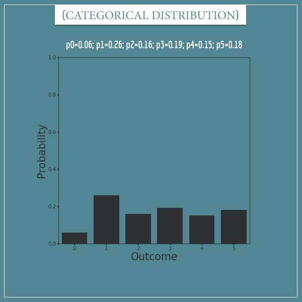
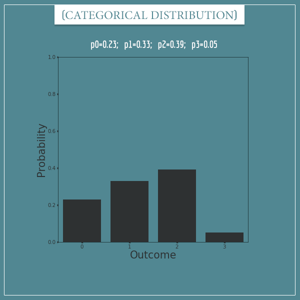
Categorical distribution plots

Here’s a categorical distribution of a random variable with 6 possible outcomes and some arbitrary values for its 6 parameters:

Here’s a categorical distribution with 4 possible outcomes:

And here’s one with only 2 possible outcomes.

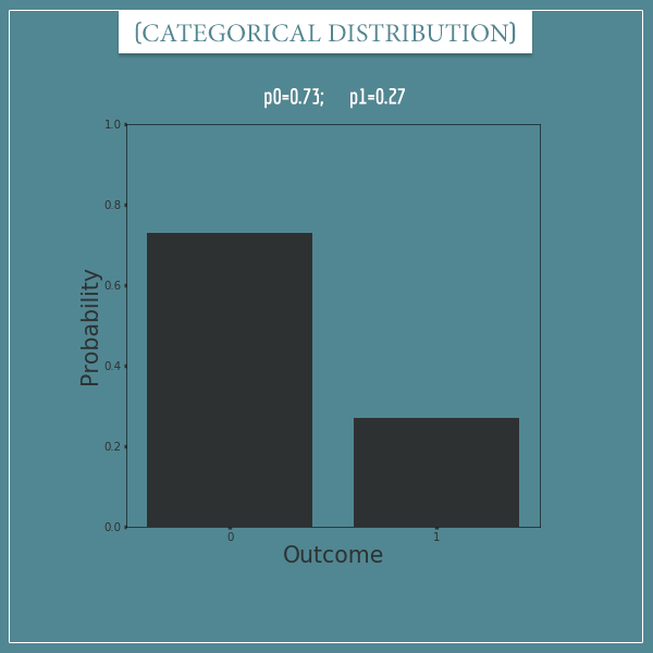
Does the last plot remind you of another distribution?

The discrete uniform distribution

Let’s finish the section on discrete probability distributions with finite sample spaces with another common distribution.

Again, imagine you have a pool of red, green, blue, and black balls. But this time they are all in the same proportion. That is, they are each 1/4 or 25% of the total number of balls in the pool. If you draw a single ball, what is the probability of it being of a particular color?

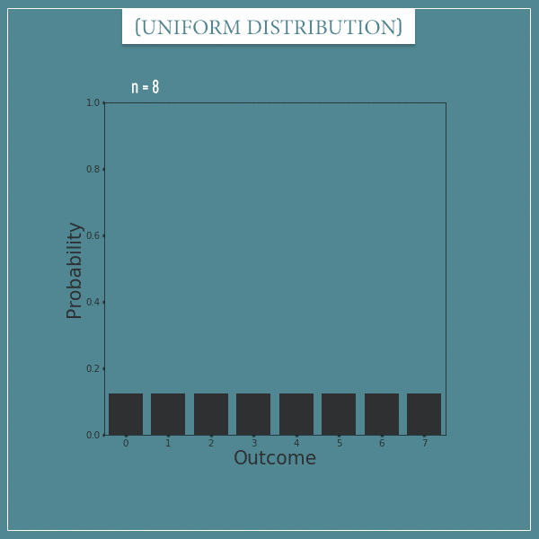
This kind of a random variable is described by the discrete uniform distribution. The random variable can have any number of possible outcomes, but they all have to be equally likely.

Hence, the discrete uniform distribution has a single parameter n which is equal to the number of possible outcomes. The probability mass function here is simply:

In a way, the discrete uniform distribution is also a special case of the categorical distribution, where all parameters are equal to the same probability (1/n).

Curious about the details? Check out my post dedicated to the uniform distribution.

Let’s take a look at a few plots.

Discrete uniform distribution plots

Here’s a uniform distribution with 8 possible outcomes:

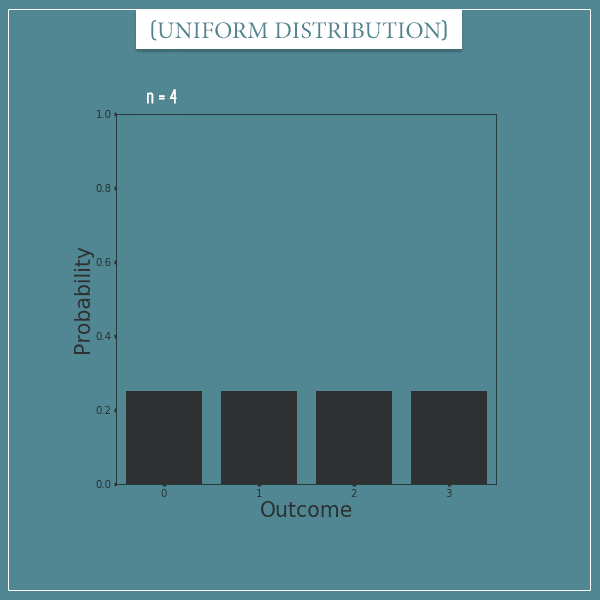
Here’s one with 4 possible outcomes:

And here’s one with only 2:

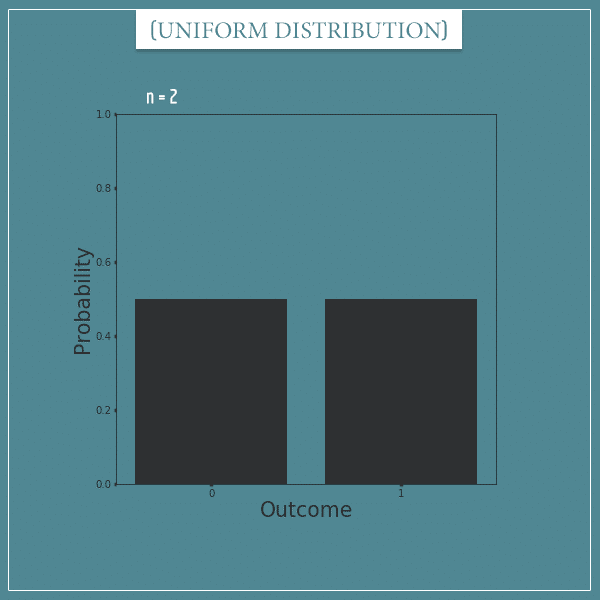
Notice that the last one is equivalent to a Bernoulli distribution with p = 0.5.

Discrete distributions with an infinite sample space

The sample spaces of all probability distributions can be represented as a subset of natural numbers. When the sample space is finite and has N elements, the subset is simply the first N natural numbers. But when the sample space has infinite elements, then it is the whole set of natural numbers.

Let’s look at a few common distributions.

The geometric distribution

You have a pool of 20% green and 80% red balls. You draw one ball and if it’s red you throw it back in the pool. Then you keep doing this until you draw the first green ball. How many red balls will you draw before the first green ball appears?

The procedure above defines the geometric distribution.

More generally, a geometric distribution describes procedures with a variable number of independent Bernoulli trials until the first “success” trial occurs. Therefore, it has a single parameter p, which is the “success” probability parameter of the underlying Bernoulli distribution.

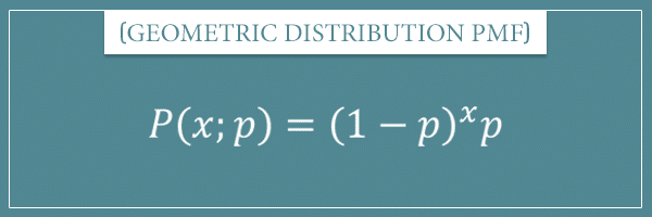
This is the probability mass function of the geometric distribution:

Let’s get some intuition about it.

In the example above, what is the probability of the outcome 0? Well, an outcome of 0 means you managed to draw a green ball on the very first trial (hence, you drew 0 red balls before the first green ball). What’s the probability of that? That’s right, it’s simply the raw probability of drawing a green ball in a single trial: 0.2. We get the same result if we plug 0 into the PMF:

   

What is the probability of drawing 1 red ball? Well, it’s the probability of drawing the green ball on the second trial, right? So, what needs to happen is exactly this: you draw a red ball on the first trial and a green ball on the second. Because the Bernoulli trials are independent, this is simply the product of the probabilities of the two outcomes:

   

We would get the same result if we plugged 1 into the PMF:

   

The general case

The outcome of drawing N red balls will always involve drawing x red balls in a row and then drawing a green ball on the very next trial. Therefore, the probability of drawing N red balls will be a product of N P(red)’s and 1 P(green). Or simply:

   

In general, getting x “failure” trials will require x “failure” trials in a row, followed immediately by a “success” trial. Hence, the probability of x “failure” trials is:

   

By the way, if you’re not sure why we’re multiplying the probabilities of independent trials, take a look at my post about compound event probabilities.

Geometric distribution plots

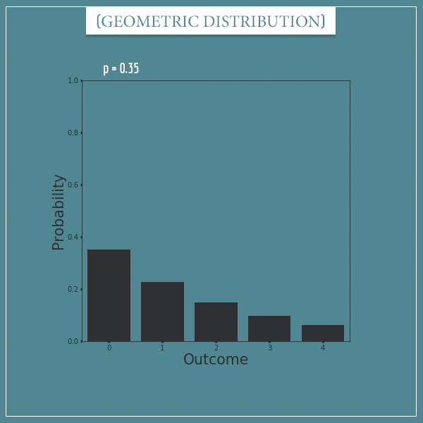
Now I’m going to show a few plots of geometric distributions. However, since the sample space here is infinite, we can’t really plot the full distribution. Because of this, I’m going to plot only the first 5 outcomes.

Here’s a geometric distribution with parameter p = 0.5:

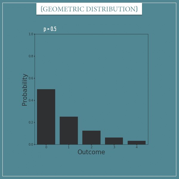
As you can see, the probabilities decrease exponentially for each additional “failure” trial. Not being able to plot infinitely many outcomes isn’t really a big problem because at some point the probabilities start getting very close to 0. So, for any geometric distribution, most of its probability mass will be concentrated over the first N outcomes, where N depends on the parameter p.

To see this, here’s a plot containing the first 10 outcomes:

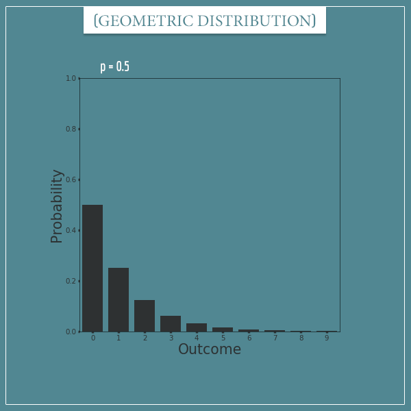
As you can see, the probabilities of the 7^th outcome and above are almost nonexistent.

Now let’s take a look at a geometric distribution with p = 0.35:

And here’s one with p = 0.75:

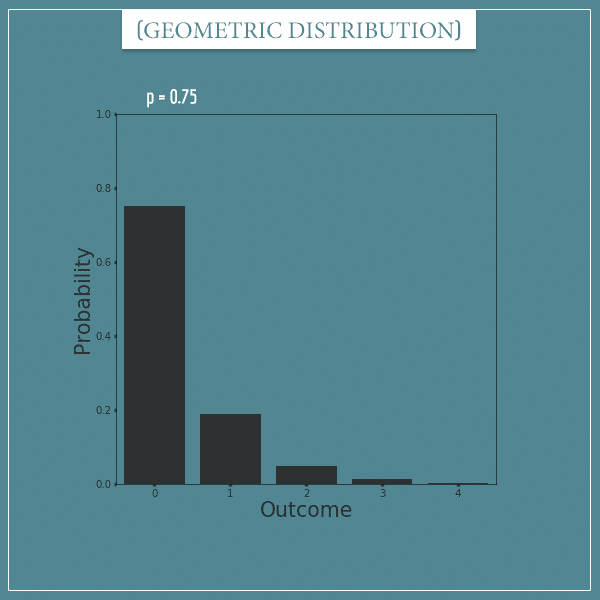
Notice that the higher the value of p is, the easier it is to get a “success” trial and, therefore, the total probability mass will be concentrated over very few of the first outcomes.

The Poisson distribution

The setting here will be somewhat different compared to the other distributions we’ve looked at so far. Again, you have a pool of green and red balls with 30% of them green. Imagine a robot that has been programmed to draw a ball once per hour and throw it back in the pool. Let’s say the robot keeps doing this forever. Then, my question is: if you pick a random day of the year, how many green balls will the robot have drawn during the entire day?

Well, this is easy enough to solve. Because there’s 24 hours in one day, the robot will have drawn exactly 24 balls from the pool. Therefore, the number of green balls will range from 0 to 24. Notice that this number will essentially have a binomial distribution with parameters p = 0.3 and n = 24.

What if the robot is drawing a ball once every minute, instead of every hour, and the percentage of green balls is only 0.5%, instead of 30%? Well, there are minutes in one day. Hence, this time we have a binomial distribution with parameters p = 0.005 and n = 1440.

What if the robot is drawing a ball once per second and the percentage of green balls is 0.0083%? Then we have a binomial distribution with p = 0.000083 and n = 86400.

Notice that in each scenario I increase the robot’s frequency of drawing a ball and decrease the percentage of green balls in the pool. Also, notice that in all three cases, on average, the robot is drawing roughly the same number of green balls per day:

   

So, what is the point here?

The Poisson distribution is a limiting case to the binomial distribution

Now stretch your imagination a bit further. Imagine the robot is drawing a ball at every single instance! In other words, imagine time as the real number line. For every real number, there’s exactly 1 ball drawn. But this is the important bit: the rate at which green balls are drawn must remain 7.2 per day. Hence, p (the probability of drawing a green ball at any specific instance) must be infinitesimally small.

In other words, imagine a binomial distribution where the parameter n approaches infinity, the parameter p approaches 0, and the product approaches 7.2.

This gives rise to a Poisson distribution with a rate parameter of 7.2. More generally, the rate parameter can be any positive real number and it is the only parameter of the distribution. It’s a convention to label this parameter with the Greek letters µ (mu) or λ (lambda). I’m going to use the former.

Here’s the probability mass function of the Poisson distribution:

The term e is Euler’s number and is approximately equal to 2.72.

This PMF is obtained when you take the limit of the expression for the binomial distribution as the parameter n approaches infinity:

   

Notice that I replaced the parameter p with µ/n. The intuition here is that the probability of a “success” trial is the total number of “success” trials in any interval of time, divided by the total number of attempts.

The main idea here is that when you take the above limit, you get the probability mass function of the Poisson distribution. The derivation isn’t too complicated, but I’m going to leave it for the post specifically dedicated to the Poisson distribution.

Poisson distribution examples

The Poisson distribution is named after the 19th century French mathematician Siméon Denis Poisson. It describes any process where a certain event occurs with a constant frequency in a fixed interval of time or space and models the probability of the number of occurrences in that interval. Also, the events must occur independently of each other and at most one event can occur at any given instance.

Even though the rate parameter is a real value, the outcomes modelled by the distribution can only be natural numbers.

Let’s come back to the robot example above. If the robot is drawing on average 7.2 green balls per day, what is the probability that it will draw, say, 5 balls? Well, we just plug the two numbers into the probability mass function:

   

So, if the average green balls is 7.2/day, the probability that exactly 5 green balls will be drawn on any given day is about 0.12.

A more realistic example is the number of emails you would get at any given hour. Say you receive about 1.4 emails per hour. What is the probability that you would get exactly 2 emails during a particular hour?

   

The assumption here is that senders of emails don’t coordinate between each other and one sender’s email doesn’t change the probability of another sender also sending an email.

Poisson distribution non-examples

The Poisson distribution wouldn’t be appropriate to use if one or more of its underlying assumptions don’t hold.

For example, you can’t use a Poisson distribution to model the number of applause events that occur in a particular minute during, say, a political speech. That is because more than one person can be applauding at any given moment. Also, when one or more people begin applauding, this usually increases the probability of more people joining them.

Another example where the Poisson distribution wouldn’t be appropriate is in modelling the number of earthquakes that occur per year in a country. The reasons are similar to the previous example — it’s possible that 2 earthquakes occur simultaneously and the occurrence of one earthquake will typically increase the probability of aftershocks.

You might be wondering if any real-world process follows a Poisson distribution exactly. That’s a good question and the answer is probably ‘no’. Often the events being modelled can’t really occur at any given instance of time, since there are physical constraints that would prevent that. For example, if you’re modelling the number of cars that pass through an intersection in any given hour, you can’t really have, say, 50 cars passing arbitrarily close in time, since the intersection has a limited capacity.

Also, sometimes you might deviate from the independence assumption as well. For example, even if emails really do arrive mostly independently of each other in your inbox, sometimes there might be a connection between them (like, if it is your birthday and you receive congratulatory emails).

However, this isn’t a big problem. Even if the pure assumptions are never actually met, if the deviation isn’t too big, the Poisson distribution will still give probabilities very close to the real ones.

Poisson distribution plots

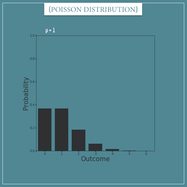
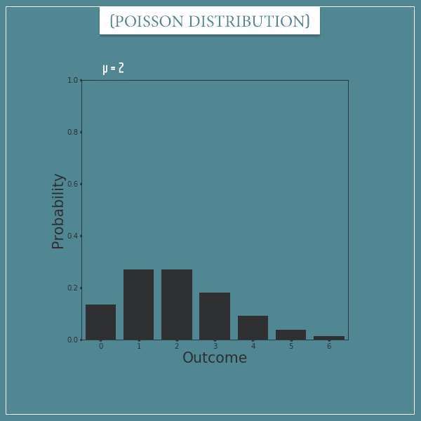
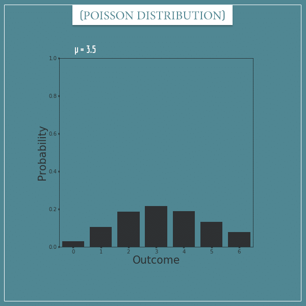
Now let’s look at some plots of Poisson distributions. Again, because the sample space is infinite, we can’t plot the full distribution, so I’m only going to show the probabilities of the first few outcomes.

Here’s a plot of a Poisson distribution with parameter µ = 1:

And here’s one with µ = 2:

Here’s one with µ = 3.5:

Finally, here’s one with µ = 10:

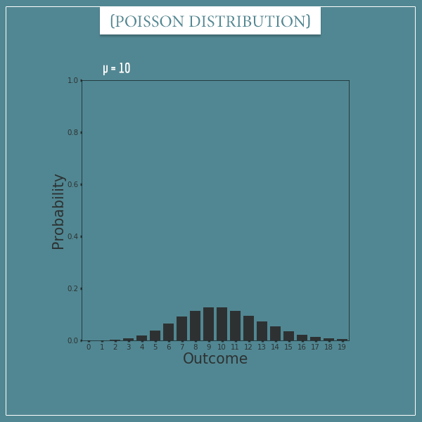
Notice how the shapes of different Poisson distributions strongly resemble the shape of a binomial distribution. This shouldn’t be too surprising, given that the Poisson distribution is defined as a limiting case to the binomial distribution. Poisson distributions with parameter µ will typically look like a narrower version (with smaller variance) of a binomial distribution with parameters n and p, where .

The Skellam distribution

And we finally come to the bonus distribution I promised to show you in the beginning.

The reason I’m showing it here isn’t so much for the mathematical intuition about the distribution itself. In fact, the derivation of its probability mass function involves some complicated mathematics that is quite beyond the scope of this post.

However, it is a discrete distribution whose domain is the whole set of integers (positive and negative) and I want to show an example of such a distribution too.

In short, a random variable having the Skellam distribution is the result of taking the difference between two independent random variables which have a Poisson distribution.

In other words, if you have any two independent Poisson distributed random variables, their difference will be Skellam distributed.

The Skellam distribution has 2 parameters: µ₁ and µ₂, which correspond to the rate parameters of the respective Poisson distributions. Here’s what the probability mass function looks like:

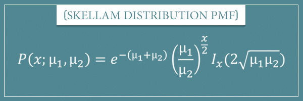
The term I_x is the so-called modified Bessel function of the first kind. It is a solution to a differential equation and, like I said, is rather complicated. In fact, it’s not a function that you would even attempt to calculate by hand, as there are easy ways to do that with computers. Consequently, don’t try to calculate the PMF itself by hand either.

Let’s say you and your friend each calculate the average emails you get per hour and for both it’s around 4. If we assume that this number is Poisson distributed, then you can use the Skellam distribution to calculate things like the probability of you receiving 2 more emails than your friend in any given hour.

Let’s look at some plots.

Skellam distribution plots

Continuing the example above, let’s look at a Skellam distribution with parameters µ₁ = 4 and µ₂ = 4:

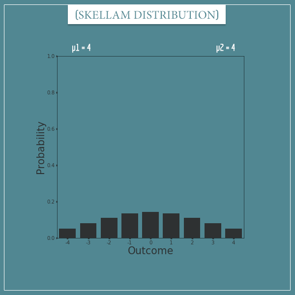
This plot should actually range from negative to positive infinity, as all integers are in the sample space.

So, it looks like for any given hour there is a probability of about 0.13 for either of you to receive 1 more email than the other person. Also, there’s a probability of about 0.14 that you would get the exact same number of emails. The probability of bigger differences will obviously be smaller.

Now, all discrete probability distributions I introduced so far had their outcomes range from 0 to a finite natural number or infinity. Can we somehow put the Skellam distribution in the same terms?

Actually, we can. Remember, the sample spaces of all discrete probability distributions can be mapped to the set of natural numbers. Just to get more intuition about this, let’s transform the plot above and map the outcomes to natural numbers:

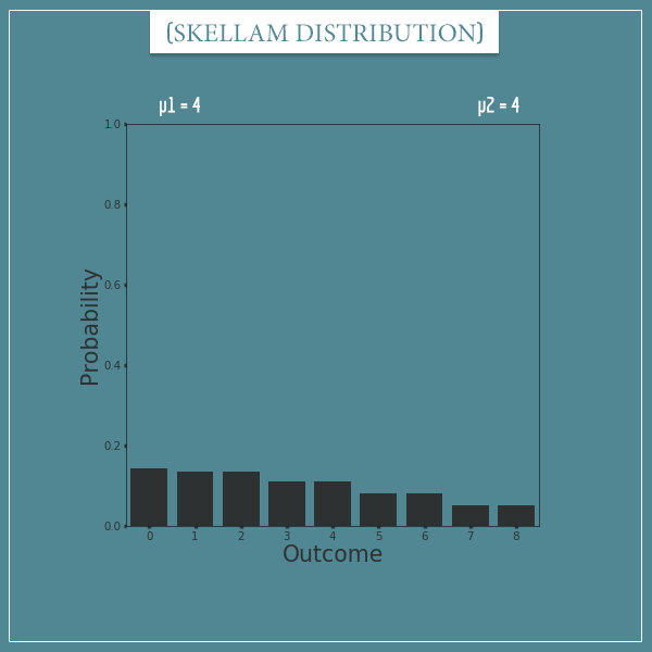
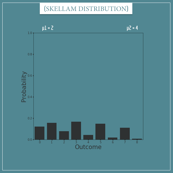
You see, after the transformation, the order of the outcomes is different but no information is lost. The 0 outcome corresponds to a difference of 0, the 1 and 2 outcomes correspond to a difference of 1, the 3 and 4 outcomes correspond to a difference of 2, and so on.

Now, you don’t have to do this transformation in real life. I’m only doing it here to give more intuition about how all discrete probability distributions can have their sample space mapped to natural numbers. However, most of the time you would work in their natural domains.

Anyway, let’s look at some more plots.

More Skellam distribution plots

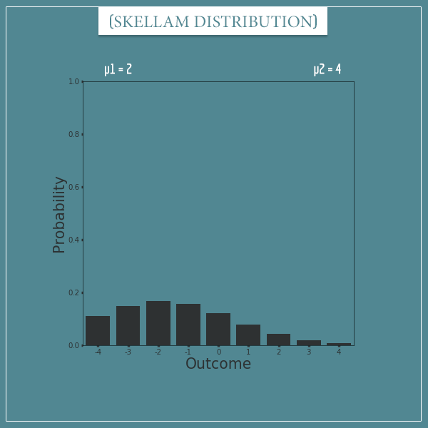
Here’s a Skellam distribution with parameters µ₁ = 2 and µ₂ = 4:

And here’s it’s transformed version:

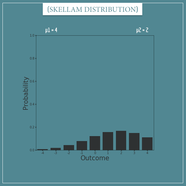
Finally, let’s look at a Skellam distribution with parameters µ₁ = 4 and µ₂ = 2:

And it’s transformed version:

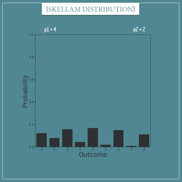
Notice how a Skellam distribution with parameters µ₁ = 4 and µ₂ = 2 is basically a mirror image of its version with parameters µ₁ = 2 and µ₂ = 4. This, of course, is going to be true for any pair of numbers.

Summary

Well, this has been a lengthy post! My goal here was to equip you with even more tools for the journey to studying and understanding the general idea of probability distributions. Unlike the previous two posts, here the focus was exclusively on discrete probability distributions.

First, I talked about the discrete nature of the sample spaces of such distributions and how they are distinguished from their continuous counterparts. The main point is simple: when you think about the sample space of a discrete random variable, you should think about natural numbers. In other words, every discrete sample space (even infinite ones) can be represented as a subset of natural numbers.

Second, I talked about the probability mass functions of discrete probability distributions and how they depend on a number of parameters. Every distribution is actually an infinite class of specific distributions, where a specific distribution is one associated with particular values of the parameters.

Finally, I introduced seven of the most commonly used discrete probability distributions. Namely, the Bernoulli, binomial, categorical, uniform, geometric, Poisson, and Skellam distributions. The first four of these have a finite sample space and the last three have an infinite sample space.

Despite its length, the post is only meant to be an overview of discrete probability distributions. I am going to go into much more detail about each of these distributions in separate posts dedicated to them. Specifically, I’m going to explain things like the exact derivation of their probability mass functions, as well as the formulas for calculating their mean and variance.

As always, let me know if you have any remarks or questions in the comment section below.

Until next time!