Intuitive Explanation of Expected Value

Expected value is another central concept in probability theory. It is a measure of the “long-term average” of a random variable (random process). I know this doesn’t sound too clear, but in this post I’m going to explain exactly what it means.

There are many areas in which expected value is applied and it’s difficult to give a comprehensive list. It is used in a variety of calculations by natural scientists, data scientists, statisticians, investors, economists, financial institutions, and professional gamblers, to name just a few.

Expected value is closely related to the concept of arithmetic mean I talked about in the post dedicated to the 3 main measures of central tendency. From another perspective, it’s also closely related to the law of large numbers which I introduced in my last post. If you’re not familiar with these concepts, I recommend reading the 2 posts for an intuitive introduction. But even if you are familiar, the posts will likely give you a different perspective and still enrich your understanding of these concepts. I also plan to use some of the intuition from the posts in explaining expected value itself. All in all, consider these two posts recommended readings.

Also, check out my post on the mean and variance of probability distributions for even more intuition on this topic. In particular, to see why the mean and the expected value of a random variable are the same thing.

And with that out of the way, let’s see what expected value is all about.

Introduction

Let’s say you work for a company that pays you a fixed salary of $7500 every month. In terms of daily expenses, you spend exactly $2500 in total every month and you put the rest in your personal bank account. Also, say you start with exactly $0 in your account on the 1^st of January. How much money do you expect to have by the 1^st of January the following year (12 months later)?

That’s easy. You put $7500 – $2500 = $5000 in your account every month. So, after 12 months you get $5000 * 12 = $60000.

Now let’s change the example a little bit. Your monthly costs and salary are still the same, but you also receive variable monthly bonuses. These bonuses depend on several market factors which are outside of your control. The lack of control and uncertainty means that the final amount you receive is no longer deterministic, but probabilistic (if you need a refresher on probabilities, check out my introductory post).

To simplify things, let’s assume the following bonus probabilities every month (each month’s bonus is independent of the rest):

• $1000 with probability 0.6
• $500 with probability 0.3
• $0 with probability 0.1

Now let’s ask the same question again: how much do you expect to have in your account after 12 months of work?

You know you’re getting $60 thousand from the fixed salary for sure (after subtracting your monthly expenses). On top of that, you’ll add an uncertain amount from the bonuses. But how much?

The obvious answer is that you don’t know for sure. And it’s true, you can’t know the exact amount with complete certainty.

For example, it’s not impossible that you get very unlucky and receive $0 in bonuses for all 12 months. In such a case, in the end you’ll still have only $60 thousand. Because the bonus probabilities are independent, the probability of getting no bonus every month is 0.1 multiplied 12 times: 0.1¹² = 0.000000000001 (take a look at my post on compound event probabilities if you’re unsure about why this is so). Very unlucky indeed! But you probably know better than to worry too much about such small probabilities.

On the other hand, you can also get very lucky and get the maximum bonus of $1000 every month, for a total of $12 thousand by the end of the year. The probability of this event is 0.6¹² ≈ 0.002. This isn’t as small as the previous case but it’s still not very impressive.

So, what amount do you expect to have in your account by the end of the year after all? We already know the lower bound to the answer is $60 thousand and the upper bound is $72 thousand. But we saw that both of these extremes have tiny probabilities, so most likely the actual amount will be somewhere between them. But is there a value within the range 60000-72000 that’s somehow more special than the others? One that you should expect more than the rest?

Yes, there is. And it’s called… the expected value.

Expected value

In this section, I’m going to show you the formal definition of expected value and how to actually calculate it. I’m also going to give you some intuition about it by showing its relationship to the arithmetic mean and the law of large numbers. As always, I’m going to give you a few examples to help everything sink in.

In fact, let’s start with our very first example and finally answer the question from the end of the previous section. I’m going to show you how to calculate the expected value in this particular example without too much explanation and I’ll give the details afterwards.

First, let’s calculate the expected bonus per month. You do this by multiplying each possible value by its respective probability and add the products.

Remember, the bonus probabilities were:

• $1000 with probability 0.6
• $500 with probability 0.3
• $0 with probability 0.1

Therefore, the expected value for 1 month is:

   

   

Then, you multiply this by 12 to get the expected bonus amount for 12 months:

   

   

So, by the end of the year, the expected value of your bonuses is $9 thousand. There’s our answer!

Of course, you add the bonuses to your fixed income to get a final expected value of $69 thousand.

See, it wasn’t hard at all. Now let’s get some deeper understanding about the calculation I just made.

Formal definition of expected value

First, let’s define the distinction between deterministic and random variables.

A deterministic variable is a variable with only one possible fixed value at any given time.  For example, your current age is a deterministic variable. To find its value, all you need to do is subtract your birth date from the current date (and optionally convert from days to years). No matter how many times you perform this measurement, you will always get the same result. In other words, your age is a fixed value (at any particular moment in time).

A random variable, on the other hand, has more than one possible values. When actually measured, the variable will take one of these values at random, each with a certain probability. For example, the side on which a coin lands is a random variable with two possible values: heads and tails, each with a probability of 0.5. Another example is the suit of a randomly drawn card from a 52-card standard deck. In this case, because there are 4 suits, the random variable has 4 possible values, each with a probability of 0.25.

Now let’s consider the general case. Let’s say that any random variable can have N number of possible values: v₁, v₂, v₃, …, v_N (N can be any number greater than 1). Let’s also denote the probabilities of the values as P(v₁), P(v₂), P(v₃), …, P(v_N).

As you might remember from the discussion in my sample space post, the probabilities of all possible values must add up to 1. That is, P(v₁) + P(v₂) + P(v₃) + … + P(v_N) = 1.

With these notations in mind, the expected value (EV) of a random variable for a single observation is given by the following expression:

   

Do you see how we applied this general formula to the salary-bonus example above? Take some time to make sure you understand the correspondence between the terms and the specific values from the example.

Well, now you have the formal definition of expected value. In the next sections, I’m going to give you some intuition about what exactly it measures and clear up some potential confusions.

Before I do that, I want to quickly introduce a mathematical notation that allows you to write the above expression in a more compact way.

The sum operator

To learn more about the sum operator, check out my post dedicated on this notation and its properties.

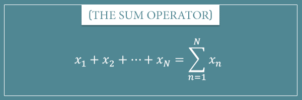
The sum operator Σ is a convenient mathematical notation for expressing the sum of a set or a sequence of values. The mathematical symbol used for the sum operator is the Greek capital letter Sigma. Take a look:

On the left-hand side of the equation, N number of values are being added up. The values are expressed as the variable x with a numerical subscript. The subscript indicates the index of the element in the sequence.

On the right-hand side, we have the same sum expressed with the sum operator. It consists of 4 parts:

• The Σ symbol, indicating a sum operation
• The n=1, indicating that the index starts from 1
• N, indicating that the index goes up to N
• x_n, which is the actual addition term

The index is incremented by 1 on each iteration (for each term of the sum). Instead of x_n, you can have an arbitrarily complex expression that consists of terms (optionally) indexed by n. Here’s how you can write the expected value of a random variable with N possible values:

To expand this, you just need to substitute the n index with the concrete numbers as you go from 1 to N. For example, for a random variable with 3 possible values, expanding the expression above would look like this:

   

Notation

Before I give you a few examples, I want to show you a common convention for a short-hand expected value notation. If you have a random variable X with N possible values , then we express the expected value of X with the capital letter E in blackboard bold:

   

Or simply or . Less commonly, you may even see it expressed as:

   

You may also hear the term “the expectation of X” which is a short way of saying “the expected value of the random variable X”.

Anyway, I’m showing you these different notations here just so you’re familiar with them and you’re not surprised if you come across them in other texts (including my posts). For the rest of this post, let’s stick with the EV(X) notation.

Examples and simulations

I want to convince you that the expected value is indeed a number that should be “expected”. Let’s confirm this with a few experimental simulations.

First, let’s look at the bonus-salary example we started with. Remember we calculated the bonus expected value for 1 month to be $750. Let’s see if that’s really the case.

In the animated plot below, you’ll see the running average of the bonuses after up to 50 months of working for the company. A running average is simply the average calculated after every month by dividing the sum of all bonuses by the number of months passed since month 0.

Click on the image to start/restart the animation.

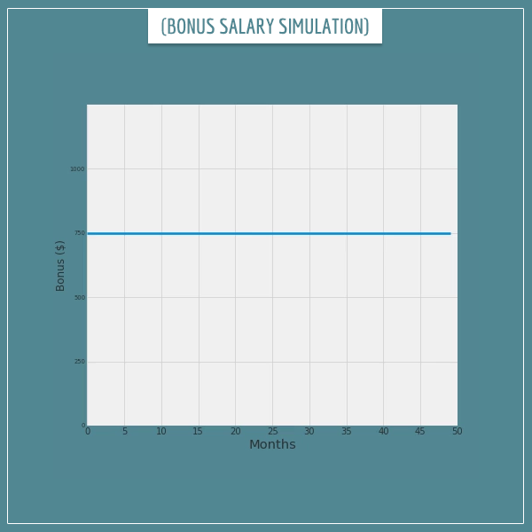
The blue line indicates the expected $750 monthly bonus. Do you see how, as the number of months increases, the average monthly bonus starts converging towards the expected value? Those of you who read my post on the law of large numbers will find this example very familiar.

Let’s run the same simulation even longer. What happens to the monthly average after working for the company for 10 years?

Click on the image to start/restart the animation.

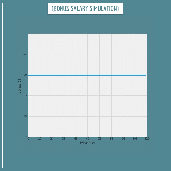
With increasing number of months, notice how the real running average deviates less and less from the expected value!

Alright, let’s look at something different. I’m going back to my favorite coin flip example.

Say someone offers you to play a game. A coin will be flipped and if it comes up heads, you win $2. If it comes up tails, you need to pay $1. Would you play the game?

Not playing the game guarantees $0 win and $0 loss. So, the way to make a choice would be by calculating the expected value of the flip and only play the game if it’s greater than $0. Let’s see:

   

Notice how one of the possible values is negative this time. A good opportunity to see this doesn’t change the expected value calculations at all.

So, since the expected value is $0.5, the game should be profitable to play. If you had the option to play it multiple times, you should take that too. In fact, how much money do you expect to have won after playing the game, say, 1000 times? The answer is $0.5*1000 = $500.

Let’s see this in action. The following 3 animated plots show the results of flipping 1 fair coin 1000 times. The first plot shows the % of heads after each flip. The next plot shows the corresponding average money won per flip. Finally, the third plot shows the total money won after each flip.

Take a look:

Click on the image to start/restart the animation.

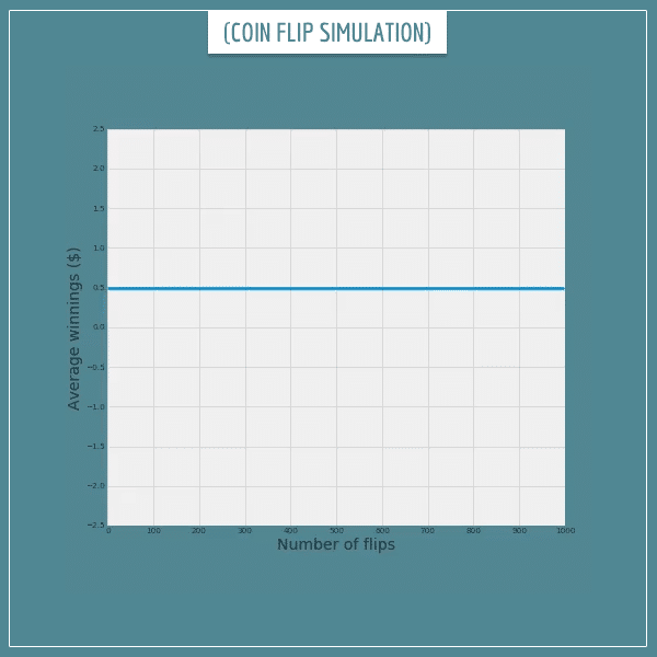
Here’s the average winnings per flip:

Click on the image to start/restart the animation.

And here’s the total winnings after each flip:

Click on the image to start/restart the animation.

All plots show exactly what we expected! The long-term average of the winnings does converge to the expected value and the total winnings get very close to the expected $500.

Of course, the actual trajectory is different every time. The empirical long-term average does fluctuate around the expected value which makes the total winnings swing up and down. But those fluctuations are local and, in the long-run, observations deviate less and less from the expectations.

In short, if someone offered you this game for 1000 flips, you can safely rely on winning some amount very close to $500.

Expected value intuition

So, why does all this work? We know individual outcomes are independent of each other and have no memory of previous outcomes. How do the values of the outcomes always manage to arrange themselves so that their long-term average keeps getting closer to the expected value?

The key to answering this question is in the relationship between expected value, arithmetic mean, and the law of large numbers.

Imagine you had a finite sequence of 1000 coin flips whose outcomes you already know. Let’s say they somehow happened to be exactly 500 heads and 500 tails. If you were playing the game from the previous section, you would immediately know how much you would win even before the game. For every heads you get $2, so $2 * 500 = $1000. For every tails you give $1 which is $1 * 500 = $500. Therefore, your bottom line from the game would be $1000 – $500 = $500.

Notice that this will be true even if you change the number of coins from 1000 to something else. As long as exactly half of the coins are heads, your final winnings will be equal to $0.5 times the number of flips.

Now imagine an infinite sequence of coin flips. Perhaps a robot has been programmed to flip a coin, pick it up, and flip it again, forever. From the law of large numbers we know that, as the number of flips increases, the heads % will get closer and closer to 50%.

Say you take a snapshot of this infinite sequence after N number of flips. If the % of heads in this sub-sequence is close to 50%, then your winnings will be very close to $0.5 * N. So, all you need to do is take a large enough N to make sure that the % of heads is really close to 50%. The law of large numbers guarantees this will work.

Another way to look at this is that, as N increases, the sequence becomes more and more like you replaced every single outcome with the long-term average (mean) of the sequence.

The same would be true in the general case where you have a random variable with more than 2 possible values. Because of the law of large numbers, you can count on the fact that the relative frequency (percentage) of each value will approach its probability.

For a discussion on the rate of convergence, check out the How large is large enough? section of my post on the law of large numbers.

Discrete versus continuous random variables

Throughout this post I’ve been assuming we’re working with discrete random variables. With continuous random variables, the sum operator is replaced by an integral. For more details on this, check out my posts on probability distributions and the mean and variance of probability distributions.

Integrals are a somewhat more complicated mathematical concept and I don’t want to make this lengthy post even lengthier. However, the idea and intuition of expected value for the continuous case is almost the same as for the discrete case. If you’re still curious about integrals and discrete vs. continuous random variables, you can read my post on zero probabilities (particularly the Integrals section). And, of course, feel free to ask any questions beyond what I covered in this or that post in the comment section below.

Summary

The expected value of a random variable is the long-term average of its possible values when values have been realized a large number of times. It is equal to the sum of the products of the values and their probabilities.

Like the law of large numbers, the expected value of a random variable is a bridge between theoretical expectations and empirical observations. The two are so closely connected that the main formulations and proofs of the law of large numbers are centered around the expected value of an arbitrary random variable.

Having a good understanding of expected value is crucial for anybody who wants to delve deeper into probability theory, statistics, and all of their related fields. You will further see how important it is in some of my future posts where I’ll discuss other theoretical concepts like probability distributions, as well as some practical application of probability theory.

I hope you found this post useful. Please share your thoughts and questions in the comment section below!