The Binomial Distribution (and Theorem): Intuitive Understanding

A skyscraper resembling a binomial distribution

Hi, everyone! And welcome to my post about the binomial distribution! Just like the Bernoulli distribution, this is one of the most commonly used and important discrete probability distributions.

This post is part of my series on discrete probability distributions.

In my previous post, I explained the details of the Bernoulli distribution — a probability distribution named after Jacob Bernoulli. This distribution represents random variables with exactly two possible outcomes, conventionally called “success” and “failure”. It’s important not only because such random variables are very common in the real world but also because the Bernoulli distribution is the basis for many other discrete probability distributions. Well, it is also the basis for the distribution from today’s post!

A portrait of Jacob Bernoulli — Jacob Bernoulli

The binomial distribution is related to sequences of fixed number of independent and identically distributed Bernoulli trials. More specifically, it’s about random variables representing the number of “success” trials in such sequences. For example, the number of “heads” in a sequence of 5 flips of the same coin follows a binomial distribution.

Just like the Bernoulli distribution, the binomial distribution could have easily been named after Jacob Bernoulli too, since he was the one who first derived it (again in his book Ars Conjectandi).

In introductory texts on the binomial distribution you typically learn about its parameters and probability mass function, as well as the formulas for some common metrics like its mean and variance. I’m going to cover all these for sure, but I also want to give you some deeper intuition about this distribution.

If you’re not familiar with discrete probability distributions in general, it’s probably better to start with my introductory post to the series.

Table of Contents

Introduction

If you’ve been following my posts, this isn’t the first time you hear the term binomial. One of the first things you probably associate it with is the binomial coefficient which I first showed you in my introductory post on combinatorics. The match in names is no coincidence — the binomial distribution is very closely related to the binomial coefficient. In fact, if you’re new to combinatorics, I strongly suggest you read this introductory post as a background for the current post.

Another mathematical concept with ‘binomial’ in its name is the binomial theorem. This is a theorem that is also closely related to the binomial distribution. And if you already understand the binomial theorem, understanding the binomial distribution will be a trivial thing.

For that reason, in the first part of this post I’m going to introduce the binomial theorem. I’m going to show you what it states and prove its statement.

In the second part, I’m going to explain the details of the binomial distribution and show you how it relates to the binomial theorem. I think this relation will give you a very good intuition for the binomial distribution, as well as enhanced intuition for the binomial theorem itself.

The binomial theorem

The binomial theorem is one of the important theorems in arithmetic and elementary algebra. In short, it’s about expanding binomials raised to a non-negative integer power into polynomials.

In the sections below, I’m going to introduce all concepts and terminology necessary for understanding the theorem. I’m obviously going to show you the theorem’s statement itself and the beautiful symmetry in it. And, so that you don’t have to blindly trust its statement, I’m also going to give you an intuitive proof for why it’s true.

Monomials, binomials, and polynomials

In mathematics it’s common to express constants with the first letters of the alphabet (a, b, c, …) and variables with the last letters (…, x, y, z). Constants are concrete numbers like 2, 5.3, and π, whereas you can think of variables as placeholders for an arbitrary number.

A monomial is a product of a constant coefficient and one or more variables, each raised to a power of some natural number (non-negative integer). The simplest possible monomial is the number 0 and any other number, like 1, 3, and 6.4, is also a monomial. You can view these examples as constants multiplied by an implicit variable (like x) raised to the power of 0. Remember, $x^0 = 1$ for any x.

Expressions of single variables like x, 2y, and 4z are also monomials where the power of the variables is 1. Here’s a couple of examples of monomials with some other powers:

$2y^5$

$5x^2y^3$

Or, (somewhat) more generally:

$dx^ay^bz^c...$

On the other hand, a binomial is a sum of exactly two monomials. For example:

$\sqrt{3}x^2 + y^4$

$xy^2 - 7z^5$

Finally, a polynomial is a sum of an arbitrary number of monomials. For example:

$x + y - z$

$2w + 3x^4 - y^2 + 7z^2$

Notice that monomials are a special case of binomials and binomials are a special case of polynomials.

Expanding binomials raised to powers

As its name suggests, the binomial theorem is a theorem concerning binomials. In particular, it’s about binomials raised to the power of a natural number. Let’s take a look at a couple of examples:

$(x + y)^2$

$(2z + 3y^4)^5$

Or, more generally:

$(cx^a + dy^b)^n$

Let’s expand the first example and get rid of the parentheses:

$(x + y)^2 = (x + y) \cdot (x + y)$

$= x^2 + xy + xy + y^2$

We can further simplify this to:

$= x^2 + 2xy + y^2$

Notice that the binomial $x + y$

raised to the power of 2 turns into a polynomial of 3 terms. As you’ll see, this is generally true for all binomials. That is, any binomial raised to a positive integer power becomes a polynomial with a number of terms one more than its power. For example, let’s expand the same polynomial but raised to the power of 3:

$(x + y)^3 = (x + y) \cdot (x + y) \cdot (x + y)$

$= (x + y) \cdot (x^2 + 2xy + y^2)$

In the second line I simply substituted the product of the first two (x + y)s with the result from the previous example. Let’s finish the expansion:

$= x^3 + 2x^2y + xy^2 + x^2y + 2xy^2 + y^3$

$= x^3 + 3x^2y + 3xy^2 + y^3$

In this case it became a polynomial of 4 terms. What if we raised it to the power of 4 or 5? Or 10? Let’s see if we can spot some general patterns.

The general case

I’m going to spare you all the hairy calculations and directly give you the results of the expansions of some powers. Here’s the expansion of $(x+y)^4$ :

$x^4 + 4x^3y + 6x^2y^2 + 4xy^3 + y^4$

And here’s the expansion of $(x+y)^5$

$x^5 + 5x^4y + 10x^3y^2 + 10x^2y^3 + 5xy^4 + y^5$

Let’s group all these results together. Take a look at the expansion of the first 6 powers of x + y (from 0 to 5):

$1$

$x + y$

$x^2 + 2xy + y^2$

$x^3 + 3x^2y + 3xy^2 + y^3$

$x^4 + 4x^3y + 6x^2y^2 + 4xy^3 + y^4$

$x^5 + 5x^4y + 10x^3y^2 + 10x^2y^3 + 5xy^4 + y^5$

And now let’s start spotting the obvious patterns.

First, notice that each term contains both x and y. Yes, even the first and last terms! The apparently missing y and x are implicitly there in the form of $y^0 = x^0 = 1$

Second, if the binomial is raised to the power of n, the number of terms in the resulting polynomial is equal to n + 1.

Third, the sum of the powers in each term is always equal to n. For example, when n = 3, the powers of the 4 terms are:

3 + 0 = 3 ( $x^3y^0$ )
2 + 1 = 3 ( $x^2y^1$ )
1 + 2 = 3 ( $x^1y^2$ )
0 + 3 = 3 ( $x^0y^3$ )

Verify for yourself that this is true for all 5 polynomials. Also, notice the elegant symmetry in all of them!

The constant coefficients

Finally, there’s one more pattern, but this one isn’t as obvious. It concerns the constant coefficients of the terms. Namely, each coefficient is equal to:

$n \choose k$

where k is the term’s position in the expression, starting from 0. For example, the first term is $n \choose 0$

, the second term is $n \choose 1$

, and so on, all the way to n (the last term).

And $n \choose k$ , of course, is the binomial coefficient I showed you in my introductory post to combinatorics:

For example, the 3rd term (position 2) from the expansion of $(x + y)^5$ is:

${5 \choose 2} = \frac{5!}{3!2!} = 10$

Which is exactly what we have for that coefficient in the expansion from the previous section. Well, now you also know why the binomial coefficient has this name!

You see that these patterns all hold true for powers up to 5. But what about higher powers? Well, this is exactly what the binomial theorem is about. Let’s finally see what it has to say.

The theorem’s statement

In a nutshell, the binomial theorem asserts the following equality:

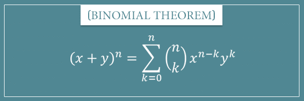
Even if it looks complicated, this formula actually states something very simple. Let’s analyze it.

On the left-hand side we have a binomial raised to the power of some n. And we already saw that when we expand a binomial raised to the power of n, we’re going to get a polynomial of n + 1 terms (at least for n up to 5). That’s why on the right hand-side there’s the sum operator representing a sum of n+1 terms. If you’re not familiar with this notation, take a look at my post about this notation and its properties.

So, to expand any binomial raised to any power, all we need to do is evaluate this sum. Let’s do an example:

$(x + y)^2 = \sum_{k=0}^{2} {2 \choose k} x^{2-k}y^k$

For the first term, we have k = 0:

$\textrm{Term}_1 = {2 \choose 0} x^{2}y^0 = x^2$

For the second term, we have k = 1:

$\textrm{Term}_2 = {2 \choose 1} x^{1}y^1 = 2xy$

Finally, for the third term we have k = 2:

$\textrm{Term}_3 = {2 \choose 2} x^{0}y^2 = y^2$

And when we add all these terms, we get the correct result:

$(x + y)^2 = x^2 + 2xy + y^2$

As an exercise, try expanding with this formula when n is 3, 4, and 5.

By the way, notice again the symmetry here. If you switched the places of x and y on the left-hand side of the formula, you’d get the exact same sum but the x’s and y’s would switch places. The powers would still run from 0 to n and from n to 0 and the sum of powers of each term would be n.

Proof and intuition

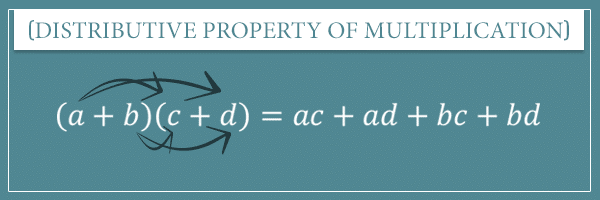
To get the intuition behind the binomial formula, we need to start from one of the fundamental arithmetic properties — the distributive property of multiplication (over addition). In short, this property states that if you multiply two binomials (or polynomials, for that matter), that’s the same as multiplying each term of the first binomial to each term of the second and summing all the products:

The formula of the distributive property of multiplication

If we apply this property to $(x + y)^2$ we get:

$(x + y)^2 = (x + y) \cdot (x + y)$

$= xx + xy + yx + yy$

And if we apply it to $(x + y)^3$

$(x + y)^3 = (x + y) \cdot (x + y) \cdot (x + y)$

$= xxx + xxy + xyx + xyy + yxx + yxy + yyx + yyy$

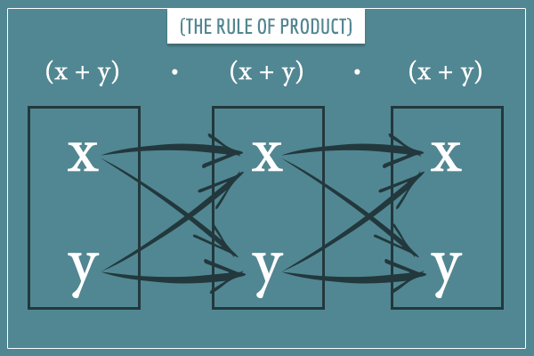
If you’ve read my introductory post on combinatorics you’ll recognize that, for any power n, there will be exactly $2^n$

such terms (by the rule of product). This is because each of the n (x + y) binomials has 2 terms. And each of the 3-character sequences are formed by picking an x or a y for each character in the sequence (from the respective binomial).

Three boxes, each with an x and y, illustrating the application of the rule of product on the binomial (x + y)

Also notice that most of the terms in the expansions above appear more than once but in a different order. For example, there’s 3 copies of $x^2y$ : xxy, xyx, and yxx. The fact that these are identical comes from another property of multiplication. Namely, the commutative property which states that, for any x and y:

$xy = yx$

Consequently, when we add all $2^3 = 8$

terms and simplify, we get integer multiples of different powers of x and y (depending on how many copies there are of that particular combination).

Deriving the binomial theorem formula

From everything we’ve seen so far, we can establish the following true statements about the raw expanded form (without any simplification) of any binomial of the form $(x + y)^n$ :

It’s a sum of $2^n$ terms, each n characters long.
Each term is a unique combination of different numbers of x’s and y’s.
The $2^n$ terms contain all possible counts of x’s and y’s (between 0 and n), as well as all possible orders of each count combination.
The counts of the x’s and y’s in each term are equal to n.

Therefore, when we express these terms as powers (for example, xyx as $x^2y$ ) and add all identical terms, we will get n + 1 terms containing all possible distributions of powers. That is, each term will contain a number of x’s and y’s from 0 to n. And because the sum of the powers of the x and the y in each term add up to n, if x’s power is k, y’s power will be n – k (and vice versa).

Okay, so far we’ve derived the following part of the binomial formula:

$(x + y)^n = \sum_{k=0}^{n} c_k x^{n-k}y^k$

Here $c_k$

is some constant coefficient which multiplies the terms $x^{n-k}y^k$

. Now, from the binomial theorem we expect $c_k$

to be:

$c_k = {n \choose k}$

But how do we prove it?

The final proof

Once we prove that $c_k = {n \choose k}$ , we will essentially complete the proof. So let’s do it!

Think about it. The general term $x^{n-k}y^k$ contains exactly k y’s, right? And the remaining n-k characters will be x’s. This means that we need to count all sequences of n-characters of which k are y’s.

But this is exactly like asking “in how many ways can we arrange n items into k slots?”, isn’t it? Consider a concrete example with n = 5 and k = 2 (3 x’s and 2 y’s). There are 5 positions for the 2 y’s to occupy. Think of these as the 5 items. And think of the 2 y’s as the 2 slots with which they can be associated.

In my post on combinatorics, I showed you this example of a (partial) 2-permutation of 5 numbers:

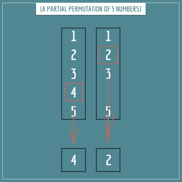
Partial permutations illustrated as choosing numbers from boxes

By analogy, here’s the same partial permutation if we assume the 5 numbers are the possible positions of the 2 y’s:

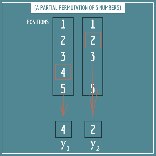
An example of a 2-permutation of the 5 possible positions in which 2 y's can occur (in a monomial of 3 x's and 2 y's)

And in the same post I explained how to count only those partial permutations that consist of the same elements (ignoring their order), which gave rise to the binomial coefficient formula.

Anyway, you can probably guess where I’m going with all this. To count all sequences of n-characters of which k are y’s (and (n – k) are x’s), we need the binomial coefficient. And since the number of such sequences is also the constant coefficient $c_k$ , we just proved that:

$c_k = {n \choose k}$

Finally, plugging this into the formula we have so far:

$(x + y)^n = \sum_{k=0}^{n} {n \choose k} x^{n-k}y^k$

So, as people like to say…

Q.E.D.

The binomial distribution

Now that we’ve analyzed the binomial theorem in detail, it’s finally time to introduce the main protagonist of this post.

The binomial distribution describes random variables representing the number of “success” trials out of n independent Bernoulli trials, where each trial has the same parameter p. In other words, where the Bernoulli trials are independent and identically distributed (IID).

Remember, a Bernoulli trial is an experiment with only 2 possible outcomes. It has a single parameter p that specifies the probability of a “success” outcome (trial). For example, a single coin flip has a Bernoulli distribution.

Say we flip the same coin three times in a row. What is the probability of getting exactly 1 “heads” (and two “tails”)? How about the probability of getting 0, 2, or 3 “heads”? Well, the binomial distribution is the discrete probability distribution which is used to answer these questions.

We already know one of the parameters of a binomial distribution — the success probability of the individual Bernoulli trials. Just like in the Bernoulli distribution, this parameter is commonly called p.

The only other parameter is the number of Bernoulli trials. It’s common to call this parameter n.

Therefore, a binomial distribution has exactly 2 parameters: p and n. In a way, the Bernoulli distribution is a special case of the binomial distribution. That is, a Bernoulli distribution is simply a binomial distribution with the parameter n = 1.

Probability mass function

Before I tell you what the probability mass function (PMF) of the binomial distribution is, I want to give you some intuition about the steps of its derivation.

Probability of a specific sequence of Bernoulli trials

Imagine we have a biased coin where p = 0.3. That is, it comes up “heads” (H) with probability 0.3 and “tails” (T) with probability 0.7. Also imagine you’re about to flip the coin 3 times. Let me ask you this: what is the probability that the three flips are going to come up HTH, exactly in this order?

First, what’s the probability that the first flip will be H? Well, it’s 0.3, right? Similarly, the probabilities of the second flip coming up T and the third coming up H are 0.7 and 0.3, respectively. Since the flips are independent of each other (the results of previous flips don’t affect the probabilities of future flips), the compound probability of the sequence HTH is the product of the individual probabilities:

$\textm{P(HTH)} = 0.3 \cdot 0.7 \cdot 0.3 = 0.063$

(If you’re not sure about this result, check out the Event (in)dependence section of my post on compound event probabilities.)

More generally, for any p, the probability of getting exactly HTH is:

$P(\textm{HTH}) = p \cdot (1 - p) \cdot p = p^2(1 - p)$

And, even more generally, to calculate the probability of any specific sequence of Bernoulli trials, you simply replace every “success” trial in the sequence with p and every “failure” trial with (1 – p). And then you simply multiply those probabilities.

Let’s label “success” trials with 1 and “failure” trials with 0. Also, for convenience, let’s define a new variable q where $q = 1 - p$ . Then if we want to calculate the probability of a sequence of Bernoulli trials like 0010101101, we would simply do:

$0010101101 \rightarrow qqpqpqppqp$

Pretty simple!

Probability of k successes out of n Bernoulli trials

Now let’s ask another question that is related to the main question of this post. If you flip a coin 3 times, what is the probability that you will get exactly 2 Hs?

To answer this question, let’s list all possible outcomes of the 3 flips. That is, let’s look at the sample space of this experiment (to make the visualization below easier to interpret, let’s assume p = 0.5):

A white square is divided into 8 equal parts, each representing an outcome of fair coin flipped 3 times

As you can see, there are 8 possible outcomes ( $2^3 = 8$ , by the rule of product). From the previous section, we know that each of these outcomes has a probability of $0.5^3 = 0.125 = \frac{1}{8}$ .

Of these 8 equally likely outcomes, the ones that satisfy the “two Hs” requirement are:

Therefore, the probability of flipping exactly two Hs is the area of the sample space that covers these 3 outcomes. And that area is nothing but the sum of probabilities of the outcomes:

$P(\textrm{2 Hs}) = P(\textrm{HHT}) + P(\textrm{HTH}) + P(\textrm{THH})$

$= 0.5^3 + 0.5^3 + 0.5^3 = 3 \cdot 0.5^3$

Now let’s generalize this result and finally derive the probability mass function of the binomial distribution.

The binomial PMF formula

Say you’re about to perform n Bernoulli trials with parameter p and want to calculate the probability of having exactly k “success” trials. The sequences that satisfy this requirement are those that have k 1’s and (n – k) 0’s, right? And the sum of their probabilities will give us the answer we’re looking for. Therefore, to calculate this probability, you need to find two things:

The probability of one of these sequences
The number of these sequences

Since each such sequence has k 1’s and (n – k) 0’s, their probabilities are:

$p^k(1-p)^{n-k}$

As for how many such sequences there are… If we have an n-character sequence of which k are 1’s, then their count is nothing but our old friend, the binomial coefficient! Therefore, the number of such sequences is ${n \choose k}$

The intuition here is identical to the one I showed you when deriving the binomial theorem. Namely, we’re counting the number of ways of arranging n items into 2 slots. Only instead of x’s and y’s, the items here are 0’s and 1’s.

Finally, we can say that the probability of having k “success” trials out of n Bernoulli trials is:

$P(\textrm{k out of n}) = {n \choose k} p^k(1-p)^{n-k}$

And we’re done! This result is the general formula for the probability mass function of a binomial distribution. Let’s make it official:

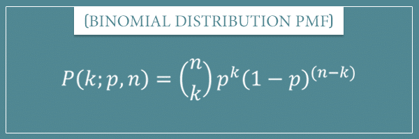
The probability mass function of a binomial distribution with input variable k and parameters p and n

The argument of the PMF

If you read the introductory post on discrete probability distributions, you might remember that I used the variable x for the argument of the function (instead of k):

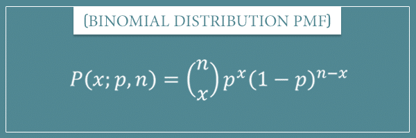
The probability mass function of a binomial distribution with input variable x and parameters p and n

In that context, it made more sense to call it x. Both for consistency and for making easier comparisons between distributions.

But in our current context, k is more descriptive and will allow for an easier comparison with the binomial theorem.

Relationship with the binomial theorem

Let’s compare the binomial distribution PMF with the formula for the binomial theorem:

Let’s do a little detective work and compare the right-hand sides of each formula. The most obvious difference is that in the binomial theorem there’s a sum, whereas the binomial distribution PMF specifies a single monomial. Let’s compare the monomials themselves.

Both start with the ${n \choose k}$ coefficient and both are followed by two terms raised to the powers k and (n – k). Other than that, the only difference is in the labels of the variables. But if we apply the variable substitutions $x = 1 - p$ and $y = p$ , we see that they are in fact identical expressions.

What if we summed the probabilities of all possible outcomes of a binomial random variable? Well, these would be the possible number of successes. So, if we have n Bernoulli trials, the possible successes will range from 0 (no successes) to n (all successes). Therefore, the sum of probabilities of all possible outcomes is:

$\sum_{k=0}^{n} {n \choose k} p^k(1-p)^{n-k}$

Now this looks exactly like the right-hand side of the binomial theorem!

Obviously, this is no coincidence. The expressions are identical because the two formulas were constructed by following an identical process. Namely, counting the number of n-character sequences, each containing different counts of two items. Whether you call those 0’s and 1’s or x’s and y’s, it really doesn’t make a difference.

To complete the intuition, let’s use the binomial theorem to actually calculate the value of this sum.

The sum of all possible outcomes

We obtained the right-hand side of the binomial theorem formula by summing all possible outcomes of a binomial random variable. But let me ask you this. What does this sum actually represent? What do you expect it to be equal to?

Well, we’re talking about the sum of all possible outcomes of a random variable, so it has to be equal to 1, right? Let’s convince ourselves that this is true. And to do that, we’re going to use the binomial theorem.

Using the variable substitutions $x = 1 - p$ and $y = p$ , the binomial theorem allows us to equate the above sum to:

$\sum_{k=0}^{n} {n \choose k} p^k(1-p)^{n-k} = ((1-p) + p)^n$

And simplifying the right-hand side yields the expected result:

$((1-p) + p)^n = (1 + 0)^n = 1^n = 1$

In other words:

$\sum_{k=0}^{n} {n \choose k} p^k(1-p)^{n-k} = ((1-p) + p)^n = 1$

Pretty neat! And notice that this holds true for any p and any n.

It’s always helpful and intuitive to independently verify what we expect to be true, isn’t it?

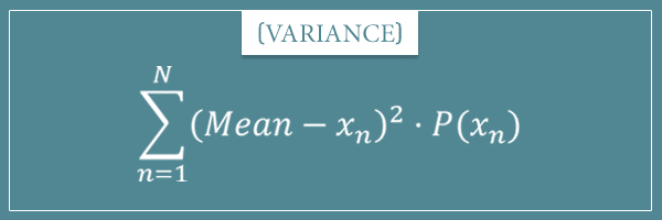
Mean and variance

Let’s remember the general formulas for the mean and variance of discrete probability distributions:

The formula for the statistical measure of central tendency called mean for discrete probability distributions

The formula for the statistical measure of dispersion called variance for discrete probability distributions

Normally, we should use these to directly derive the specific formulas for the binomial distribution. And we can. But this post already has a lot of calculations and derivations and I don’t want to overwhelm you.

That’s why I decided to write a bonus post that specifically deals with the rigorous proof of the formulas I’m about to show you. Here I’m only going to show you a more intuitive derivation.

The main intuition is that a binomial experiment consists of a series of independent Bernoulli experiments (trials). Here are two true statements (without proof) about the sum of a set of independent random variables:

Its mean (expected value) is the sum of the individual means (expected values).
Its variance is the sum of the individual variances.

And a binomial trial is essentially the sum of n individual Bernoulli trials, each contributing a 1 or a 0. Therefore, to calculate the mean and variance of a binomial random variable, we simply need to add the means and variances of the n Bernoulli trials.

Remember the mean and variance formulas of the Bernoulli distribution:

$\textrm{Mean} = p$

$\textrm{Variance} = p(1-p)$

Since we’re adding n of those, the mean and variance of a binomial distribution are simply:

$\textrm{Mean} = np$

$\textrm{Variance} = np (1-p)$

I hope these results make intuitive sense. But if you want to see a more rigorous proof, check out my bonus proof post.

Binomial distribution plots

By now you should have a pretty good intuition about the binomial distribution. But to give you an even better picture of the concept, in the final section of this post I want to show you some plots. These plots have different values for the n and p parameters and will give you a good feeling for what the binomial distribution generally looks like.

For example, here’s a plot of a binomial distribution with parameters p = 0.5 and n = 5:

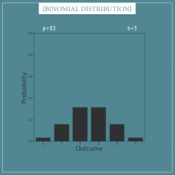
This distribution represents things like the number of heads out of 5 fair coin flips. Applying the binomial PMF, we can calculate the probability of, say, 2 “success” trials:

$P(k=2; p=0.5, n=5) = \binom{5}{2} \cdot 0.5^5 = 0.3125$

Pretty simple, isn’t it? Here are the probabilities for the remaining possible outcomes:

0: 0.03125
1: 0.15625
2: 0.3125
3: 0.3125
4: 0.15625
5: 0.03125

And the mean of the distribution is $np = 5 \cdot 0.5 = 2.5$ . Notice how the distribution is symmetric around this mean.

Compare this to a binomial distribution with the same p but n = 10:

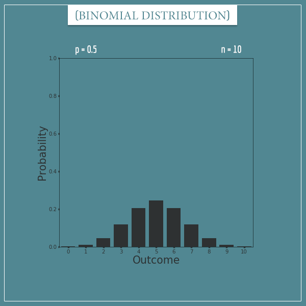
A plot of a binomial distribution with parameters: p = 0.5 and n = 10

Here the mean is $np = 10 \cdot 0.5 = 5$ and the symmetry is again around this value.

Finally, this is what a binomial distribution with p = 0.65 and n = 7 looks like:

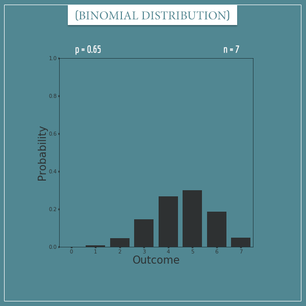
A plot of a binomial distribution with parameters: p = 0.65 and n = 7

The mean is $np = 7 \cdot 0.65 = 4.55$ and notice how $p \neq 0.5$ breaks the symmetry.

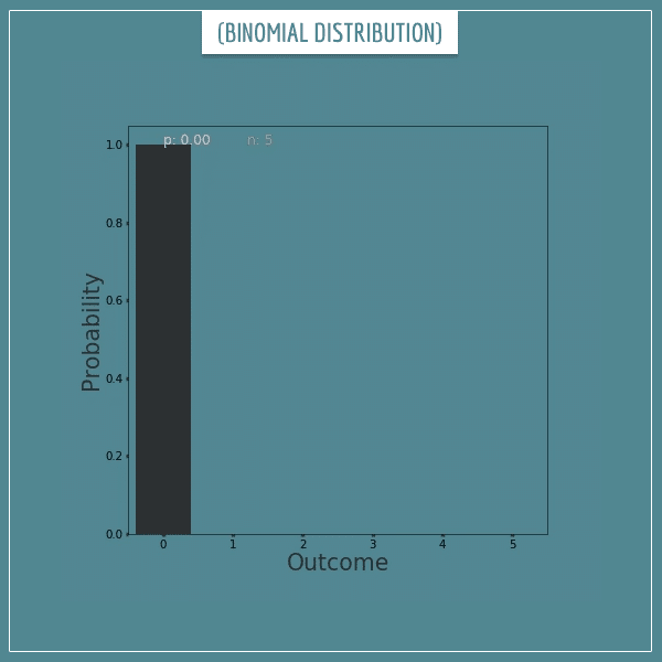
There are infinitely many binomial distributions defined by the parameters n and p. This is true for any distribution whose parameters can take an infinite number of values.

To get a better intuition, let’s take a look at a few animations.

Binomial distribution animations

In my previous post, I showed you an animation that went through the full range of values for the parameter p of the Bernoulli distribution. Now let’s look at a few similar animations for a binomial distribution when n is 5, 10, and 15. Click on each of the 3 images below to see the animations:

A simulation of consecutive coin flips with a rolling mean of heads

In all these plots you can see that the distribution is symmetric around the mean only when p = 0.5. This symmetry comes directly from the symmetry in the binomial theorem itself. When $p \neq 0.5$ , the symmetry is broken because outcomes start receiving disproportionate “boost” from the product of p’s representing them.

For example, when $p < 0.5$ , the distribution will tend to be skewed towards the outcomes below the mean. Similarly, when $p > 0.5$ , the distribution is skewed towards outcomes greater than the mean.

Summary

In today’s post I gave you a detailed and (hopefully) intuitive picture of the binomial theorem and the binomial distribution. I showed you how the derivation of their formulas follows an identical logic.

The new concepts I introduced in this post are monomials, binomials, and polynomials. The binomial theorem states that expending any binomial raised to a non-negative integer power n gives a polynomial of n + 1 terms (monomials) according to the formula:

$(x + y)^n = \sum_{k=0}^{n} {n \choose k} x^{n-k}y^k$

On the other hand, the binomial distribution describes a random variable whose value is the number (k) of “success” trials out of n independent Bernoulli trials with parameter p. The probability mass function we derived is:

$P(k; p, n) = {n \choose k} p^k(1-p)^{n-k}$

I showed you its relationship to the binomial theorem when we used it to prove that the sum of all possible outcomes of a binomial random variable is equal to 1:

$\sum_{k=0}^{n} {n \choose k} p^k(1-p)^{n-k} = ((1-p) + p)^n = 1$

Finally, I showed you an intuitive derivation for the mean and variance of the binomial distribution:

$\textrm{Mean} = np$

$\textrm{Variance} = np (1-p)$

If you’re not satisfied and want to see a more rigorous derivation, check out my bonus post where I show the formal derivation and proof of these two formulas.

As always, if you had any difficulties with any part of this post, leave your questions in the comment section below.

Until next time!

Comments

haveaniceday says

September 28, 2020 at 8:23 am

Love your explanations, pls keep posting articles

Swaroop Kumar says

October 27, 2021 at 12:28 am

That’s an amazing read of a post passionately written! Thank you so much!

Varun says

November 20, 2021 at 3:07 am

Crystal clear!! Please keep on writing such amazing posts. Thank you!!

David says

December 25, 2021 at 5:45 am

Excellent!!! I just finished a statistics course and immediately went on the internet to look for an article just like this. You did not disappoint.

Imash Shanelka says

November 2, 2022 at 9:22 am

Thank you very much sir !!! what a nice explanation

Introduction

The binomial theorem

Monomials, binomials, and polynomials

Expanding binomials raised to powers

The general case

The constant coefficients

The theorem’s statement

Proof and intuition

Deriving the binomial theorem formula

The final proof

The binomial distribution

Probability mass function

Probability of a specific sequence of Bernoulli trials

Probability of k successes out of n Bernoulli trials

The binomial PMF formula

The argument of the PMF

Relationship with the binomial theorem

The sum of all possible outcomes

Mean and variance

Binomial distribution plots

Binomial distribution animations

Summary

Comments

Leave a Reply Cancel reply