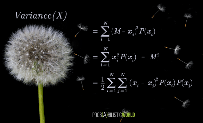
Alternative Variance Formulas and Their Derivation

The equations of three alternative variance formulas

In today’s post I want to show you two alternative variance formulas to the main formula you’re used to seeing (both on this website and in other introductory texts).

Not only do these alternative formulas come in handy for the derivation of certain proofs and identities involving variance, they also further enrich our intuitive understanding of variance as a measure of dispersion for a finite population or a probability distribution.

I also want to use this post as an exercise for performing useful manipulations of expressions involving the sum operator. This mathematical notation and its properties was the topic of my last post and today I want to show you real examples of how you can apply thеse properties in certain derivations.

As a quick reminder, the sum operator is a mathematical notation for expressing sums of elements of a sequence.

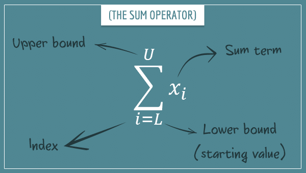
A capital letter Sigma representing the sum operator, along with its four components: the index, the lower bound, the upper bound, and the sum term (labeled with arrows)

You expand such expressions by iterating over the values of the index i between the lower and the upper bound, plugging each value into the sum term and adding it to the existing sum:

$\sum_{i=L}^{U} x_i = x_{L} + x_{L+1} + ... + x_{U}$

Before I move to the actual alternative formulas, I want to give a quick review of some properties and formulas I’ve derived in previous posts.

Table of Contents

Overview of sum operator and variance formulas

In deriving the alternative variance formulas, I’m going to use the following four sum operator properties. I wrote them as labeled equations so that I can easily refer to them later on:

Multiplying a sum by a constant:

(1) $\begin{equation*}c \sum_{i=L}^{U} x_i = \sum_{i=L}^{U} c x_i\end{equation*}$

Adding or subtracting sums with the same number of terms:

(2) $\begin{equation*}\sum_{i=L}^{U} x_i \pm \sum_{i=L}^{U} y_i = \sum_{i=L}^{U} (x_i \pm y_i)\end{equation*}$

Multiplying sums:

(3) $\begin{equation*}\sum_{i=L_1}^{U_1} x_i \cdot \sum_{j=L_2}^{U_2} y_j = \sum_{i=L_1}^{U_1} \sum_{j=L_2}^{U_2} x_i \cdot y_j\end{equation*}$

Changing the order of double sums:

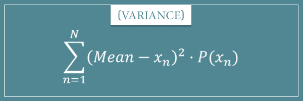
(4) $\begin{equation*}\sum_{i=L_1}^{U_1} \sum_{j=L_2}^{U_2} x_{i, j} = \sum_{j=L_2}^{U_2} \sum_{i=L_1}^{U_1} x_{i, j}\end{equation*}$

As far as variance is concerned, I first talked about it in my post about the different measures of dispersion in the context of finite populations. The formula I showed you in that post was:

The formula for the statistical dispersion measure called variance

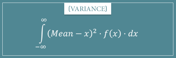
And in my post about the mean and variance of probability distributions I showed you the following formula for discrete probability distributions:

The formula for the statistical measure of dispersion called variance for discrete probability distributions

As well as this formula for continuous probability distributions:

The formula for the statistical measure of dispersion called variance for continuous probability distributions

I’m first going to derive the alternative formulas for discrete probability distributions and after that I’m going to show you their finite population and continuous distribution counterparts.

By the way, notice that I used n instead of i as the index variable in the images above. In other posts I’ve also used the letter k. Obviously the choice of letter doesn’t matter, but for the rest of this post I’m going to stick to the convention of using i for the index (as well as j, when we’re dealing with double sums).

Other background information

Besides these properties and formulas, I’m also generally going to rely on the properties of arithmetic operations. If you’re not familiar with them, check out my post on the topic.

It’s probably also useful to get familiar with the concept of expected value (if you’re not already), which you can do by reading my introductory post on expected value. In parts of this post I’m going to use one of the notations I showed you there. Namely, for a random variable X, the expected value (or mean) of the variable is expressed as:

(5) $\begin{equation*}\mathop{\mathbb{E}[X] = \sum_{i=1}^{N} x_i \cdot P(x_i)\end{equation*}$

That is, with the capitalized and blackboard bold version of the letter E.

Oh, and one last thing. In the derivations below, I’m occasionally going to make use of a special case of the binomial theorem (which I explained in my post on the binomial distribution). Namely, the following identity which holds true for any two real numbers x and y:

(6) $\begin{equation*}(x-y)^2 = x^2 - 2xy + y^2\end{equation*}$

And, with all this in mind, let’s finally get to the meat of today’s topic.

Alternative variance formula #1

For those of you following my posts, I already used this formula in the derivation of the variance formula of the binomial distribution. Here it is:

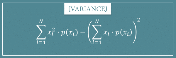
An alternative formula for the statistical dispersion measure called variance

In words, it says that the variance of a random variable X is equal to the expected value of the square of the variable minus the square of its mean. Let’s first prove that this formula is identical to the original one and then I’m going to briefly discuss it.

If you’re confused by what the expected value of $X^2$ means, take a look at this section from my post on mean and variance of probability distributions.

Derivation

Let’s start with the general formula for the variance of a discrete probability distribution where we write M for the mean:

$\textrm{Variance(X)} = \sum_{i=1}^{N} (M - x_i)^2 \cdot P(x_i)$

First, using equation (6), let’s expand the squared difference inside the sum:

$(M - x_i)^2 = M^2 - 2Mx_i + x_i^2$

Then we can rewrite the variance formula as:

$\textrm{Variance(X)} = \sum_{i=1}^{N} (M^2 - 2Mx_i + x_i^2) \cdot P(x_i)$

$= \sum_{i=1}^{N} \left( M^2 \cdot P(x_i) - 2Mx_i \cdot P(x_i) + x_i^2 \cdot P(x_i) \right)$

In the last line, I simply used the distributive property of multiplication over addition to put the $P(x_i)$

inside the parentheses.

Splitting the big sum into simpler sums

Now, using equation (2), we can rewrite the above formula as:

$\textrm{Variance(X)} = \sum_{i=1}^{N} \left( M^2 \cdot P(x_i) - 2Mx_i \cdot P(x_i) + x_i^2 \cdot P(x_i) \right)$

$= \sum_{i=1}^{N} M^2 \cdot P(x_i) - \sum_{i=1}^{N} 2Mx_i \cdot P(x_i) + \sum_{i=1}^{N} x_i^2 \cdot P(x_i)$

Finally, using equation (1), we can take out the constant terms outside the sums and rewrite this as:

$M^2 \cdot \sum_{i=1}^{N} P(x_i) - 2M \cdot \sum_{i=1}^{N} x_i \cdot P(x_i) + \sum_{i=1}^{N} x_i^2 \cdot P(x_i)$

Notice that:

$\sum_{i=1}^{N} P(x_i) = 1$

Because this is the sum of probabilities of all possible values (which by definition is equal to 1). Furthermore:

$\sum_{i=1}^{N} x_i \cdot P(x_i) = M$

Which is simply the mean of the distribution from equation (5)!

Finally:

$\sum_{i=1}^{N} x_i^2 \cdot P(x_i) = \mathbb{E}[X^2]$

Which is simply the expected value of $X^2$

Final steps

Plugging these three into the full expression for the variance formula, we get:

$\textrm{Variance(X)} = M^2 \cdot 1 - 2M \cdot M + \mathop{\mathbb{E}[X^2]$

$= M^2 - 2M^2 + \mathop{\mathbb{E}[X^2]$

And adding the $M^2$

terms:

$\textrm{Variance(X)} = \mathop{\mathbb{E}[X^2] - M^2$

$= \mathop{\mathbb{E}[X^2] - \mathop{\mathbb{E}[X]^2$

The last two expressions are identical. In various articles you’ll typically see the second one and, admittedly, it looks more elegant. But I personally prefer the first one because I find it a bit more readable.

And we’re done! Now we can finally state the following with confidence:

$\textrm{Variance(X)} = \sum_{i=1}^{N} (M - x_i)^2 \cdot P(x_i) = \mathop{\mathbb{E}[X^2] - M^2$

Discussion

In my first post on variance, I told you that any measure of dispersion needs to be a number between 0 and infinity (∞). Furthermore, a measure has to be sensitive to how much the data is spread. It should be 0 if and only if there is absolutely no variability in the data and it should grow as the data becomes more spread (or dispersed).

The main formula of variance is consistent with these requirements because it sums over squared differences between each value and the mean. If all values are equal to some constant c, the mean will be equal to c as well and all squared differences will be equal to 0 (hence the variance will be 0). And as the values get farther from the mean, the square of their deviations also grows.

Random variables with zero mean

To understand the intuition behind the first alternative variance formula, imagine a random variable whose mean is equal to 0. Let’s denote it as $X_o$ . Quick question: what is the variance of $X_o$ ?

Well, if the mean is zero, by definition $\mathbb{E}[X_o] = 0$ and the alternative formula reduces to:

$\textrm{Variance(}X_o\textrm{)} = \mathop{\mathbb{E}[X_o^2] - \mathbb{E}[X_o]^2 = \mathop{\mathbb{E}[X_o^2] - 0^2$

$= \mathop{\mathbb{E}[X_o^2]$

Actually, the main formula would reduce to the same thing as well but the point is that, if the mean is 0, the variance simply measures the expected squared deviations from 0. The farther apart the values are from 0, the bigger their spread. And, hence, the larger the variance will be. So far, it’s intuitive enough.

Adding a constant to a zero-mean variable

Now let’s create a new random variable by adding some constant M to $X_o$ :

$Y = X_o + M$

Notice that the mean of this new random variable is going to be M (this should be pretty intuitive, but try to prove it as an exercise):

$\mathop{\mathbb{E}[Y] = \mathop{\mathbb{E}[X_o + M] = M$

But since we’re adding a constant, we’re simply shifting the distribution to the left or to the right (depending on whether the constant is a positive or a negative number). We’re not actually changing its variability in any way, which means that its variance should remain the same:

$\textrm{Variance(}X_o + M\textrm{)} = \textrm{Variance(}X_o\textrm{)}$

This is indeed a property of variance that can be easily proved, which I’ll do in a future post (along with other properties). Though feel free to try it yourself as an exercise.

Now let’s write an expression for the variance of Y:

$\textrm{Variance(Y)} = \textrm{Variance(}X_o + M\textrm{)} = \mathop{\mathbb{E}[(X_o + M)^2] - \mathop{\mathbb{E}[X_o + M]^2$

$= \mathop{\mathbb{E}[(X_o + M)^2] - M^2$

And since we know that the variance of $X_o + M$

should be equal to $\mathop{\mathbb{E}[X_o^2]$

$\textrm{Variance(Y)} = \mathop{\mathbb{E}[(X_o + M)^2] - M^2 = \mathop{\mathbb{E}[X_o^2]$

From which it follows that:

$\mathop{\mathbb{E}[(X_o +M)^2] = \mathop{\mathbb{E}[X_o^2] + M^2$

That is, this line of reasoning lead us to the conclusion that adding a constant M to a random variable whose mean is 0 is the same as adding $M^2$

to the expected value of the square of the variable. To complete our mathematical intuition, let’s prove this independently:

$\mathop{\mathbb{E}[(X_o +M)^2] = \mathop{\mathbb{E}[(X_o^2 +2X_oM + M^2)]$

$= \mathop{\mathbb{E}[X_o^2] + 2M\mathop{\mathbb{E}[X_o] + \mathop{\mathbb{E}[M^2]$

And since $\mathop{\mathbb{E}[X_o] = 0$

and $\mathop{\mathbb{E}[M^2] = M^2$

, we get:

$\mathop{\mathbb{E}[(X_o +M)^2] = \mathop{\mathbb{E}[X_o^2] + M^2$

Which confirms the intuition. I know I skipped a few intermediate steps, but you should be able to fill those in. If you’re having any difficulties, let’s discuss this in the comment section below.

Alternative variance formula #2

Now let’s look at the second alternative variance formula I promised to show you.

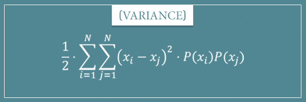
What’s interesting about it is that it makes no reference to the mean of the random variable! Let’s first look at its derivation and then we’ll discuss its interpretation as well.

Derivation

We can derive this alternative variance formula starting from the main formula, but I don’t want to interrupt our current journey. Since the last thing we did was derive the first alternative variance formula, let’s continue from there:

$\textrm{Variance(X)} = \mathop{\mathbb{E}[X^2] - \mathop{\mathbb{E}[X]^2$

I first want to rewrite the two terms as double sums. The short answer to why I’m doing this is because I want to use equation (2) and join them back into a single sum. You’ll see the full reason shortly.

Rewriting the terms as double sums

Let’s start with the left term:

$\mathop{\mathbb{E}[X^2] = \sum_{i=1}^{N} x_i^2 \cdot p(x_i) = \sum_{i=1}^{N} x_i^2 \cdot p(x_i) \cdot 1$

All I did here is multiply the sum term by 1, which obviously doesn’t change its value. It looks a little silly, doesn’t it? Well, to see why I’m doing this, let’s rewrite the number 1 itself in the following way:

$1 = \sum_{j=1}^{N} p(x_j)$

We basically did the same thing in one of the steps in the previous section but in the opposite direction — the sum of all elements of a sample space is always equal to 1. Notice, however, that we’re using a different letter for the index — j instead of i. Now let’s replace the 1 inside the sum term with this sum:

$\mathop{\mathbb{E}[X^2] = \sum_{i=1}^{N} \left(x_i^2 \cdot p(x_i) \cdot \sum_{j=1}^{N} p(x_j) \right)$

Because the $x_i^2 \cdot p(x_i)$

part of the sum term is independent of j, it’s a constant with respect to the inner sum. Which means we can move it inside to obtain the following double sum:

$\mathop{\mathbb{E}[X^2] = \sum_{i=1}^{N} \sum_{j=1}^{N} x_i^2 \cdot p(x_i) \cdot p(x_j)$

So far, so good! Now let’s also start writing the right term of the variance formula as a double sum:

$\mathop{\mathbb{E}[X]^2 = \left(\sum_{i=1}^{N} x_i \cdot p(x_i)\right)^2 = \sum_{i=1}^{N} x_i \cdot p(x_i) \cdot \sum_{j=1}^{N} x_j \cdot p(x_j)$

All I did was write the second power more explicitly as a product. However, notice that again I used j as an index for the second sum! We can do that, right? Regardless of what letter you choose for the index, the sum remains the same. But now equation (3) (and the commutative property of multiplication) allows us to rewrite this product of sums as the following double sum:

$\sum_{i=1}^{N} x_i \cdot p(x_i) \cdot \sum_{j=1}^{N} x_j \cdot p(x_j) = \sum_{i=1}^{N} \sum_{j=1}^{N} x_i \cdot x_j \cdot p(x_i) \cdot p(x_j)$

Joining the terms into a single double sum

So far, we wrote the two terms of the variance formula as the following double sums:

$\mathop{\mathbb{E}[X^2] = \sum_{i=1}^{N} \sum_{j=1}^{N} x_i^2 \cdot p(x_i) \cdot p(x_j)$

$\mathop{\mathbb{E}[X]^2 = \sum_{i=1}^{N} \sum_{j=1}^{N} x_i \cdot x_j \cdot p(x_i) \cdot p(x_j)$

And when we plug these into the variance formula, we get:

$\textrm{Variance(X)} = \mathop{\mathbb{E}[X^2] - \mathop{\mathbb{E}[X]^2$

$= \sum_{i=1}^{N} \sum_{j=1}^{N} x_i^2 \cdot p(x_i) \cdot p(x_j) - \sum_{i=1}^{N} \sum_{j=1}^{N} x_i \cdot x_j \cdot p(x_i) \cdot p(x_j)$

But now, using equation (2), we can merge the two double sums into one:

$\textrm{Variance(X)} = \sum_{i=1}^{N} \sum_{j=1}^{N} \left(x_i^2 \cdot p(x_i) \cdot p(x_j) - x_i \cdot x_j \cdot p(x_i) \cdot p(x_j)\right)$

And using the distributive property of multiplication, we can factor out $p(x_i) \cdot p(x_j)$

to finally obtain the formula:

$\textrm{Variance(X)} = \sum_{i=1}^{N} \sum_{j=1}^{N} (x_i^2 - x_i \cdot x_j) \cdot p(x_i) \cdot p(x_j)$

This is already an interesting expression! It tells us that the variance can also be written as this double sum whose terms are differences of the square of an element and the product of that element with another element.

But we’re not done yet. Let’s see if we can get this into an even more elegant shape.

Switching the indices

Notice that it was kind of arbitrary that we expressed the first index as i and the second as j. If we had started with j instead, an equally valid alternative representation of the formula above is:

$\textrm{Variance(X)} = \sum_{j=1}^{N} \sum_{i=1}^{N} (x_j^2 - x_j \cdot x_i) \cdot p(x_j) \cdot p(x_i)$

But now, using equation (4), as well as the commutative property of multiplication, we can rewrite this as:

$\sum_{i=1}^{N} \sum_{j=1}^{N} (x_j^2 - x_i \cdot x_j) \cdot p(x_i) \cdot p(x_j)$

From which we conclude that this particular representation of the variance formula has a twin representation:

$\textrm{Variance(X)} =\sum_{i=1}^{N} \sum_{j=1}^{N} (x_i^2 - x_i \cdot x_j) \cdot p(x_i) \cdot p(x_j)$

$= \sum_{i=1}^{N} \sum_{j=1}^{N} (x_j^2 - x_i \cdot x_j) \cdot p(x_i) \cdot p(x_j)$

Keep these in mind because we’re going to use them in the final steps of the derivation.

The final steps

Now I want to apply another mathematical trick. I want to write an expression for twice the variance as addition:

$2\cdot \textrm{Variance(X)} = \textrm{Variance(X)} + \textrm{Variance(X)}$

However, for each $\textrm{Variance(X)}$

term, I want to write a different version of the formula we derived above (the twin formulas):

$2\cdot \textrm{Variance(X)} = \sum_{i=1}^{N} \sum_{j=1}^{N} (x_i^2 - x_i \cdot x_j) \cdot p(x_i) \cdot p(x_j) + \sum_{i=1}^{N} \sum_{j=1}^{N} (x_j^2 - x_i \cdot x_j) \cdot p(x_i) \cdot p(x_j)$

I’m doing this because now we can merge back the two sums. And after also factoring out the common terms, we get:

$2\cdot \textrm{Variance(X)} = \sum_{i=1}^{N} \sum_{j=1}^{N} (x_i^2 - 2 \cdot x_i \cdot x_j + x_j^2) \cdot p(x_i) \cdot p(x_j)$

Now, do you notice anything familiar about the part inside the parentheses? It looks exactly like the right-hand side of equation (6), no? Using this equation, we can finally write the formula as:

$2\cdot \textrm{Variance(X)} = \sum_{i=1}^{N} \sum_{j=1}^{N} (x_i - x_j)^2 \cdot p(x_i) \cdot p(x_j)$

There you have it. Now all we need to do is divide both sides of this equation by 2 in order to get a formula for the variance that looks like this:

$\textrm{Variance(X)} = \frac{1}{2} \cdot \sum_{i=1}^{N} \sum_{j=1}^{N} (x_i - x_j)^2 \cdot p(x_i) \cdot p(x_j)$

Whoa! Look at this, it’s pretty isn’t it? We have expressed the variance of a random variable X in terms of the sum of the squared differences between all possible pairs of elements of its sample space. Not only that, this formula makes absolutely no reference to the mean of the distribution!

Discussion

Let’s do a quick recap. According to the original formula, the variance of a random variable X is equal to the expected value of the squared difference between X and its mean. And, according to the first alternative formula we derived, the same measure can be expressed as the difference between the expected value of the square of the variable and the square of its mean.

Now, after some additional manipulations, we found out that the exact same measure can also be expressed in terms of the square of differences between all possible values of X. Well, half of that, since we’re dividing the double sum by 2.

Apart from allowing us to calculate the variance without having to calculate the mean first, this formula offers additional insight about what the variance represents. Turns out, measuring dispersion through sums of squared differences from the mean is the same as summing all squared differences between the values themselves. The intuition behind dividing by two is that each pair of values is counted twice by the standard double sum, since:

$(x_i - x_j)^2 = (x_j - x_i)^2$

In other words, not dividing by two would overestimate the variance by a factor of 2. Although, notice that in principle $2 \cdot \textrm{Variance(X)}$

is just as valid measure of dispersion as $\textrm{Variance(X)}$

. Still, if you’re somewhat bothered by the $\frac{1}{2}$

factor, we can also write this formula as:

$\textrm{Variance(X)} = \sum_{i=1}^{N} \sum_{j=i+1}^{N} (x_i - x_j)^2 \cdot p(x_i) \cdot p(x_j)$

Here we removed the $\frac{1}{2}$

factor but the index of the inner sum doesn’t start from 1. Instead, it starts from the current index of the outer sum + 1. If you remember, I talked about such expressions in a section of my post about the sum operator. Starting the inner sum’s index at i+1 instead of 1 leads to adding the square of differences between each pair only once and we no longer need the $\frac{1}{2}$

factor in front. Which probably makes the formula somewhat more elegant.

I’m going to revisit this formula in my post on measures of dispersion of categorical random variables (that is, ones with a categorical probability distribution). As you’ll see, this will offer further intuition about variance in general.

Now, before I conclude this post, I want to show you how all these alternative variance formulas translate to situations where, instead of a discrete distribution, we’re dealing with a continuous one or a finite population.

Generalizing alternative variance formulas

In my first and introductory post on variance, I gave you this formula for any finite collection of numbers:

Which, using equation (1), can be rewritten as:

$\textrm{Variance(X)} = \sum_{i=1}^{N} (M - x_i)^2 \cdot \frac{1}{N}$

Basically, the $p(x_i)$

term is replaced by $\frac{1}{N}$

because each value in the collection has an equal chance of being selected.

So, this is how the main variance formula translates from discrete probability distributions to finite populations. The two new variance formulas we derived today translate in the exact same way.

Finite populations

For discrete distributions, we derived:

$\textrm{Variance(X)} = \sum_{i=1}^{N} x_i^2 \cdot p(x_i) - \left(\sum_{i=1}^{N} x_i \cdot p(x_i)\right)^2$

$\textrm{Variance(X)} = \frac{1}{2} \cdot \sum_{i=1}^{N} \sum_{j=1}^{N} (x_i - x_j)^2 \cdot p(x_i) \cdot p(x_j)$

If we now replace the $p(x_i)$

and $p(x_j)$

terms with $\frac{1}{N}$

again, the finite population versions of these two formulas become:

$\textrm{Variance(X)} = \frac{1}{N} \cdot \sum_{i=1}^{N} x_i^2 - \frac{1}{N^2} \cdot \left(\sum_{i=1}^{N} x_i \right)^2$

$\textrm{Variance(X)} = \frac{1}{2N^2} \cdot \sum_{i=1}^{N} \sum_{j=1}^{N} (x_i - x_j)^2$

Continuous distributions

Alright, what about continuous probability distributions? Remember the main variance formula for an arbitrary probability density function f(x):

To translate the first alternative formula, we simply need to calculate the expected value of the squares of X and subtract the square of the mean from it:

$\textrm{Variance(X)} = \mathop{\mathbb{E}[X^2] - \mathop{\mathbb{E}[X]^2$

Which in the language of integrals translates to:

$\textrm{Variance(X)} = \int_{-\infty}^{\infty} x^2 \cdot f(x) \cdot \,dx - \left( \int_{-\infty}^{\infty} x \cdot f(x) \cdot \,dx \right)^2$

The idea is that the sum operator turns into an integral where the $x_i$

term is replaced by the variable x multiplied by dx (since that’s the variable we’re integrating over). And, of course, the probability mass function $P(x_i)$

is replaced with the probability density function $f(x)$

For the second alternative variance formula, we replace the double sum with a double integral, as well as the $x_i$ and $x_j$ terms with x and y:

$\textrm{Variance(X)} = \frac{1}{2} \cdot \int_{-\infty}^{+\infty} \int_{-\infty}^{+\infty} (x-y)^2 \cdot f(x) \cdot f(y) \cdot \,dx \cdot \,dy$

Since we’re integrating over x and y, for both we have the corresponding dx and dy terms. Finally, the $P(x_i) \cdot P(y_j)$

product is replaced with $f(x) \cdot f(y)$

For those of you not familiar with integrals, you’ll gain more intuition about the above formulas when I write my post dedicated to this topic. For now, I’m giving you these translations without a formal proof just so you have the big picture.

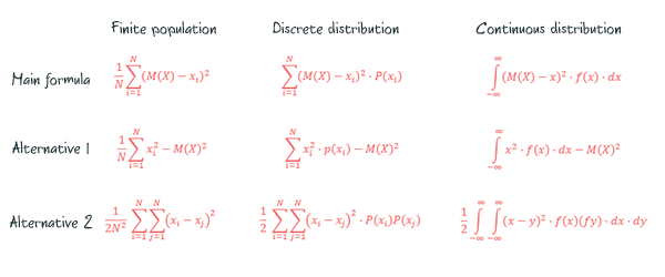
Summary

In today’s post I showed you two alternative variance formulas which are both useful and insightful. I derived these formulas for discrete probability distributions and later showed you their finite population and continuous distribution versions. Here’s a table that summarizes all these results:

Three versions of the same variance formula for finite populations, discrete distributions, and continuous distributions

I hope this post was also a useful exercise in manipulating expressions involving the sum operator. Some of the things we did weren’t exactly trivial but they are things you’ll come across in other mathematical texts quite often. If you understood everything in this post, this should boost your confidence in your ability to understand many other (even more advanced) derivations.

Overview of the derivation steps

Here’s a summary of the derivation steps of the first alternative formula:

$\textrm{Variance(X)} = \sum_{i=1}^{N} (M - x_i)^2 \cdot P(x_i) = \sum_{i=1}^{N} (M^2 - 2Mx_i + x_i^2) \cdot P(x_i)$

$= M^2 \cdot \sum_{i=1}^{N} P(x_i) - 2M \cdot \sum_{i=1}^{N} x_i \cdot P(x_i) + \sum_{i=1}^{N} x_i^2 \cdot P(x_i) = M^2 - 2M^2 + \mathop{\mathbb{E}[X^2]$

Finally:

$\textrm{Variance(X)} = \mathop{\mathbb{E}[X^2] - M^2 = \mathop{\mathbb{E}[X^2] - \mathop{\mathbb{E}[X]^2$

And here’s a summary of the steps for the second alternative variance formula:

$\mathop{\mathbb{E}[X^2] = \sum_{i=1}^{N} \sum_{j=1}^{N} x_i^2 \cdot p(x_i) \cdot p(x_j)$

$\mathop{\mathbb{E}[X]^2 = \sum_{i=1}^{N} \sum_{j=1}^{N} x_i \cdot x_j \cdot p(x_i) \cdot p(x_j)$

In the beginning we simply wrote the terms of the first alternative formula as double sums. Then:

$\textrm{Variance(X)} = \sum_{i=1}^{N} \sum_{j=1}^{N} x_i^2 \cdot p(x_i) \cdot p(x_j) - \sum_{i=1}^{N} \sum_{j=1}^{N} x_i \cdot x_j \cdot p(x_i) \cdot p(x_j)$

$= \sum_{i=1}^{N} \sum_{j=1}^{N} (x_i^2 - x_i \cdot x_j) \cdot p(x_i) \cdot p(x_j)$

$= \sum_{i=1}^{N} \sum_{j=1}^{N} (x_j^2 - x_i \cdot x_j) \cdot p(x_i) \cdot p(x_j)$

Finally, we multiplied the variance by 2 to get the following identity:

$2\cdot \textrm{Variance(X)} = \sum_{i=1}^{N} \sum_{j=1}^{N} (x_i^2 - x_i \cdot x_j) \cdot p(x_i) \cdot p(x_j) + \sum_{i=1}^{N} \sum_{j=1}^{N} (x_j^2 - x_i \cdot x_j) \cdot p(x_i) \cdot p(x_j)$

$= \sum_{i=1}^{N} \sum_{j=1}^{N} (x_i^2 - 2 \cdot x_i \cdot x_j + x_j^2) \cdot p(x_i) \cdot p(x_j) = \sum_{i=1}^{N} \sum_{j=1}^{N} (x_i - x_j)^2 \cdot p(x_i) \cdot p(x_j)$

And after dividing both sides of the equation by 2:

$\textrm{Variance(X)} = \frac{1}{2} \cdot \sum_{i=1}^{N} \sum_{j=1}^{N} (x_i - x_j)^2 \cdot p(x_i) \cdot p(x_j)$

Well, I hope you learned something new (and useful) today. As always, if you got stuck somewhere or have any other questions (or insights of your own), feel free to drop a comment in the comment section below!

Comments

The Carkcah says

April 20, 2022 at 10:02 am

Very cool ! THX

Sam S says

October 20, 2022 at 11:55 am

This is an amazing post!

I am struggling with one part…in the equation after the following sentence in the “Alternative variance formula #1” section:

Which is simply the mean of the distribution from equation (5)!

I do not understand how the left side of the term equates to E[X^2]

Overview of sum operator and variance formulas

Other background information

Alternative variance formula #1

Derivation

Splitting the big sum into simpler sums

Final steps

Discussion

Random variables with zero mean

Adding a constant to a zero-mean variable

Alternative variance formula #2

Derivation

Rewriting the terms as double sums

Joining the terms into a single double sum

Switching the indices

The final steps

Discussion

Generalizing alternative variance formulas

Finite populations

Continuous distributions

Summary

Overview of the derivation steps

Comments

Leave a Reply Cancel reply