
This is a bonus post for my main post on the binomial distribution. Here I want to give a formal proof for the binomial distribution mean and variance formulas I previously showed you.
This post is part of my series on discrete probability distributions.
In the main post, I told you that these formulas are:
![\[ \textrm{Mean} = np \]](https://www.probabilisticworld.com/wp-content/ql-cache/quicklatex.com-e19a441b1a73454e00462f50cb002d8a_l3.png "Rendered by QuickLaTeX.com")
![\[ \textrm{Variance} = np (1-p) \]](https://www.probabilisticworld.com/wp-content/ql-cache/quicklatex.com-71b70d7022e7d329e8d832f5a09b1625_l3.png "Rendered by QuickLaTeX.com")
For which I gave you an intuitive derivation. The intuition was related to the properties of the sum of independent random variables. Namely, their mean and variance is equal to the sum of the means/variances of the individual random variables that form the sum. We could prove this statement itself too but I don’t want to do that here and I’ll leave it for a future post.
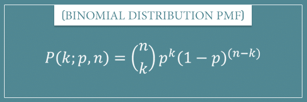
Instead, I want to take the general formulas for the mean and variance of discrete probability distributions and derive the specific binomial distribution mean and variance formulas from the binomial probability mass function (PMF):
To do that, I’m first going to derive a few auxiliary arithmetic properties and equations. We’re going to use those as pieces of the main proofs. But their usefulness is much bigger and you can apply them for many other derivations.
I think this post will be a great exercise for those of you who don’t have much experience in formal derivations of mathematical formulas. I’m going to be as explicit as I can and try to not skip even the smallest steps. So, don’t be scared by the quantity of equations in this post. I promise, you’ll be able to follow everything!
And if you happen to get stuck somewhere, I’m going to answer all of your questions in the comments. Don’t hesitate to ask me anything.
Table of Contents
Auxiliary properties and equations
To make it easy to refer to them later, I’m going to label the important properties and equations with numbers, starting from 1. These identities are all we need to prove the binomial distribution mean and variance formulas. The derivations I’m going to show you also generally rely on arithmetic properties and, if you’re not too experienced with those, you might benefit from going over my post breaking down the main ones.
The first two equations are two important identities involving the sum operator which I proved in my recent post on the topic:
(1) 
(2) 
Second, in another recent post on different variance formulas I showed you the following alternative variance formula for a random variable X with mean M:
(3) ![\begin{equation*}\textrm{Variance(X)} = \mathop{\mathbb{E}[X^2] - M^2\end{equation*}](https://www.probabilisticworld.com/wp-content/ql-cache/quicklatex.com-ec97a97ddcd132ad822eff2a689e112c_l3.png "Rendered by QuickLaTeX.com")
It’s a pretty nice formula used in many derivations, not just the ones I’m about to show you (for more intuition, check out the link above). According to this formula, the variance can also be expressed as the expected value of
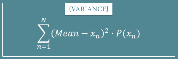
 minus the square of its mean. As a reminder (and for comparison), here’s the main variance formula:
 ![\[\textrm{Variance(X)} = \sum_{n=1}^{N} (M - x_n)^2 \cdot P(x_n)\]](https://www.probabilisticworld.com/wp-content/ql-cache/quicklatex.com-ea19686f01c188a9418e05028bb85ec1_l3.png "Rendered by QuickLaTeX.com")
A property of the binomial coefficient
Finally, I want to show you a simple property of the binomial coefficient which we’re going to use in proving both formulas. Remember the binomial coefficient formula:
![\[ \binom{n}{k} = \frac{n!}{(n-k)!k!} \]](https://www.probabilisticworld.com/wp-content/ql-cache/quicklatex.com-04df7dca9ca4e5c66954495f8eabae4d_l3.png "Rendered by QuickLaTeX.com")
The first useful result I want to derive is for the expression
 . Let’s apply the formula to this expression and simplify:
 ![\[ \binom{n-1}{k-1} = \frac{(n-1)!}{((n-1) - (k-1))!(k-1)!} \]](https://www.probabilisticworld.com/wp-content/ql-cache/quicklatex.com-0eb721e11fa27b84936a4322636c8167_l3.png "Rendered by QuickLaTeX.com")
![\[ = \frac{(n-1)!}{(n-k)!(k-1)!} \]](https://www.probabilisticworld.com/wp-content/ql-cache/quicklatex.com-9c5fdef0ef20fa38200c7b9f01ee149d_l3.png "Rendered by QuickLaTeX.com")
Therefore:
![\[\binom{n-1}{k-1} = \frac{(n-1)!}{(n-k)!(k-1)!}\]](https://www.probabilisticworld.com/wp-content/ql-cache/quicklatex.com-639bd86b6eaed820103ab4ea3e19a554_l3.png "Rendered by QuickLaTeX.com")
Now let’s do something else. One of the simplest properties of the factorial function is:
![\[ x! = x \cdot (x - 1)! \]](https://www.probabilisticworld.com/wp-content/ql-cache/quicklatex.com-d1f406bdf11644f6bffb63928c5a2024_l3.png "Rendered by QuickLaTeX.com")
I want to use this to derive the main property of binomial coefficients we’re interested in here. First, let’s use it to rewrite the right-hand side in the following way:
![\[ \binom{n}{k} = \frac{n!}{(n-k)!k!} = \frac{n(n-1)!}{(n-k)!k(k-1)!} \]](https://www.probabilisticworld.com/wp-content/ql-cache/quicklatex.com-78ecf1d305d7b6b0bc01d3ca23585b22_l3.png "Rendered by QuickLaTeX.com")
And using the commutative property of multiplication (
 ), we can rewrite the right-hand side as:
 ![\[ \frac{n}{k} \cdot \frac{(n-1)!}{(n-k)!(k-1)!} \]](https://www.probabilisticworld.com/wp-content/ql-cache/quicklatex.com-64ae723aef47415f7d12759399be9da8_l3.png "Rendered by QuickLaTeX.com")
Now let’s say we start with another expression:
 . Using the result above, we can equate it to:
 ![\[ k \cdot \binom{n}{k} = k \cdot \frac{n}{k} \cdot \frac{(n-1)!}{(n-k)!(k-1)!} \]](https://www.probabilisticworld.com/wp-content/ql-cache/quicklatex.com-daa00c3531331db1183cb84ecc4b6f57_l3.png "Rendered by QuickLaTeX.com")
![\[ = n \cdot \frac{(n-1)!}{(n-k)!(k-1)!} \]](https://www.probabilisticworld.com/wp-content/ql-cache/quicklatex.com-8a2defd89ad106bf32038e7233c5469c_l3.png "Rendered by QuickLaTeX.com")
In the last step, I simply canceled out the two k’s. Finally, using
 (derived above), we get the following identity:
 (4) 
And with all that out of the way, let’s get to the main proofs of today’s post!
Mean of binomial distributions derivation
Well, here we reach the main point of this post! Let’s use these equations and properties to derive the formulas we’re interested in.
First is the mean. Here’s the general formula again:

Let’s plug in the binomial distribution PMF into this formula. To be consistent with the binomial distribution notation, I’m going to use k for the argument (instead of x) and the index for the sum will naturally range from 0 to n. So, with ![M(K) = \mathop{\mathbb{E}[K]](https://www.probabilisticworld.com/wp-content/ql-cache/quicklatex.com-2b1ac212da17a24c0c77ee49b0e303d5_l3.png "Rendered by QuickLaTeX.com") in mind, we have:
in mind, we have:
![\[ \mathop{\mathbb{E}[K] = \sum_{k=0}^{n} k \cdot \binom{n}{k} p^k(1-p)^{n-k} \]](https://www.probabilisticworld.com/wp-content/ql-cache/quicklatex.com-654a83f4b1642be770e0dc6ba8f76fa6_l3.png "Rendered by QuickLaTeX.com")
But notice that when k = 0 the first term is also zero and doesn’t contribute to the overall sum. Therefore, we can also write the formula by having the index start from k = 1:
![\[ \mathop{\mathbb{E}[K] = \sum_{k=1}^{n} k \cdot \binom{n}{k} p^k(1-p)^{n-k} \]](https://www.probabilisticworld.com/wp-content/ql-cache/quicklatex.com-c1977dfcb9bc630ebc5f8b278d8bb610_l3.png "Rendered by QuickLaTeX.com")
Now let’s see how we can manipulate the right-hand side to get the desired
![\mathop{\mathbb{E}[K] = np](https://www.probabilisticworld.com/wp-content/ql-cache/quicklatex.com-7216c9b4f5a10b302a5b3ec75fa846a6_l3.png "Rendered by QuickLaTeX.com") . Let’s do the proof step by step.
. Let’s do the proof step by step.
Proof steps
The first step in the derivation is to apply the binomial property  from equation (4) to the right-hand side:
![\[ \mathop{\mathbb{E}[K] = \sum_{k=1}^{n} n \cdot \binom{n-1}{k-1} p^k(1-p)^{n-k} \]](https://www.probabilisticworld.com/wp-content/ql-cache/quicklatex.com-3c4a0cea39ac8e910c833aa382638248_l3.png "Rendered by QuickLaTeX.com")
![\[ = n \cdot \sum_{k=1}^{n} \binom{n-1}{k-1} p^k(1-p)^{n-k} \]](https://www.probabilisticworld.com/wp-content/ql-cache/quicklatex.com-1511e10ed38433c40af6fd263e97f843_l3.png "Rendered by QuickLaTeX.com")
In the second line, I simply used equation (1) to get n out of the sum operator (because it doesn’t depend on k).
Next, we’re going to use the product rule of exponents:
![\[ x^n \cdot x^m = x^{n+m} \]](https://www.probabilisticworld.com/wp-content/ql-cache/quicklatex.com-fcac0c08ec449fa0879304b174cc7e77_l3.png "Rendered by QuickLaTeX.com")
A special case of this rule is:
![\[ x^n = x \cdot x^{n-1} \]](https://www.probabilisticworld.com/wp-content/ql-cache/quicklatex.com-05485ca0e6896c59c1520c47ae86709d_l3.png "Rendered by QuickLaTeX.com")
And we’re going to use it to rewrite
 as
as  :
: ![\[ \mathop{\mathbb{E}[K] = n \cdot \sum_{k=1}^{n} \binom{n-1}{k-1} pp^{k-1}(1-p)^{n-k} \]](https://www.probabilisticworld.com/wp-content/ql-cache/quicklatex.com-c47f74d8267065dab0b7f2576539baf1_l3.png "Rendered by QuickLaTeX.com")
![\[ = np \cdot \sum_{k=1}^{n} \binom{n-1}{k-1} p^{k-1}(1-p)^{n-k} \]](https://www.probabilisticworld.com/wp-content/ql-cache/quicklatex.com-7b4ac340096b142406ccca74a6dd5e6b_l3.png "Rendered by QuickLaTeX.com")
Again, in the last line I simply took out the constant term p outside of the sum operator. Finally, let’s apply the identity
 to the exponent of (1 – p) (you’ll see why we do this in a moment):
 ![\[ \mathop{\mathbb{E}[K] = np \cdot \sum_{k=1}^{n} \binom{n-1}{k-1} p^{k-1}(1-p)^{(n - 1) - (k - 1)} \]](https://www.probabilisticworld.com/wp-content/ql-cache/quicklatex.com-b79a869f568a88ae8ce60059169f0f45_l3.png "Rendered by QuickLaTeX.com")
The final proof
Believe it or not, we’re almost done here. Notice that, after the last manipulation, there’s a lot of terms like n – 1 and k – 1 inside the sum operator. To make the expression a little more readable, let’s rewrite it by applying the following variable substitutions:
![\[ n - 1 = m \]](https://www.probabilisticworld.com/wp-content/ql-cache/quicklatex.com-a2d01a605cda44cdbc55e8ebec1e6104_l3.png "Rendered by QuickLaTeX.com")
![\[ k - 1 = j \]](https://www.probabilisticworld.com/wp-content/ql-cache/quicklatex.com-697c4dccebfb4078d7b4128e8be44f9e_l3.png "Rendered by QuickLaTeX.com")
This results in:
![\[ \mathop{\mathbb{E}[K] = np \cdot \sum_{j=0}^{m} \binom{m}{j} p^j(1-p)^{m-j} \]](https://www.probabilisticworld.com/wp-content/ql-cache/quicklatex.com-dcf67bf4015cf7700ebe3d13942a7dc0_l3.png "Rendered by QuickLaTeX.com")
Here j starts from 0 because j = k – 1 (the k index used to start from 1 before the variable substitution). And because the number of terms in the sum must be preserved, the index runs until n – 1 = m.
Now, do you recognize the term inside the sum operator?
![\[ \binom{m}{j} p^j(1-p)^{m-j} \]](https://www.probabilisticworld.com/wp-content/ql-cache/quicklatex.com-2c5de157d22966689e464621d09cb93b_l3.png "Rendered by QuickLaTeX.com")
It looks exactly like the binomial PMF, doesn’t it? Only k has been replaced with j and n with m. And since the sum is from 0 to m, this is simply the sum of probabilities of all outcomes, right? Then, by definition:
![\[ \sum_{j=0}^{m} \binom{m}{j} p^j(1-p)^{m-j} = 1 \]](https://www.probabilisticworld.com/wp-content/ql-cache/quicklatex.com-68cc13ae12ef1fbb77e751c714917925_l3.png "Rendered by QuickLaTeX.com")
And plugging this last result into what we have so far, we get:
![\[ = np \cdot 1 = np \]](https://www.probabilisticworld.com/wp-content/ql-cache/quicklatex.com-e4f4ffa8bd6c8b226bc28fb3c0f53200_l3.png "Rendered by QuickLaTeX.com")
Therefore, we can now confidently state:
![\[ \mathop{\mathbb{E}[K] = np \]](https://www.probabilisticworld.com/wp-content/ql-cache/quicklatex.com-a9ac9d3dc97b394aa0132377f1b1eebb_l3.png "Rendered by QuickLaTeX.com")
Q.E.D.
Variance of binomial distributions derivation
Now it’s time to prove the variance formula. Remember the general variance formula for discrete probability distributions:
Like before, for the argument of the PMF I’m going to use k, instead of x. Furthermore, I’m going to use the alternative variance formula from equation (3) we derived earlier:
![\[ \textrm{Variance(K)} = \mathop{\mathbb{E}[K^2] - \mathop{\mathbb{E}[K]^2 \]](https://www.probabilisticworld.com/wp-content/ql-cache/quicklatex.com-1b994aa0b1332bdb75136e6d30a4dc38_l3.png "Rendered by QuickLaTeX.com")
Using the result from the previous section:
And we can plug in
![\mathop{\mathbb{E}[K]^2 = (np)^2](https://www.probabilisticworld.com/wp-content/ql-cache/quicklatex.com-a5c97b422667fd3311a80d21fefcea62_l3.png "Rendered by QuickLaTeX.com") to get:
to get: ![\[ \textrm{Variance(K)} = \mathop{\mathbb{E}[K^2] - (np)^2 \]](https://www.probabilisticworld.com/wp-content/ql-cache/quicklatex.com-e860d6ff19884d237cb90099a08124c9_l3.png "Rendered by QuickLaTeX.com")
We already solved half of the problem! Now let’s focus on the
![\mathop{\mathbb{E}[K^2]](https://www.probabilisticworld.com/wp-content/ql-cache/quicklatex.com-4953e92084c62628632d5cefb773cd3b_l3.png "Rendered by QuickLaTeX.com") term. Using the binomial PMF, this expected value is equal to:
term. Using the binomial PMF, this expected value is equal to: ![\[ \mathop{\mathbb{E}[K^2] = \sum_{k=0}^{n} k^2 \cdot \binom{n}{k} p^k(1-p)^{n-k} \]](https://www.probabilisticworld.com/wp-content/ql-cache/quicklatex.com-c7ed807f68edf3219b8cba9e95517a34_l3.png "Rendered by QuickLaTeX.com")
Like before, when k = 0 the first term in the sum becomes zero again. So we can similarly write the same sum with the index starting from 1:
![\[ \mathop{\mathbb{E}[K^2] = \sum_{k=1}^{n} k^2 \cdot \binom{n}{k} p^k(1-p)^{n-k} \]](https://www.probabilisticworld.com/wp-content/ql-cache/quicklatex.com-938949827d4bcd5103e5ea663d21ef7b_l3.png "Rendered by QuickLaTeX.com")
With this setup, let’s start with the actual proof. The focus is going to be on manipulating the last equation. When we’re done with that, we’re going to plug in the final result into the main formula.
You’ll see that the mathematical tricks we use are going to be very similar to the ones we used in the previous proof.
Proof steps
First, using equation (4), let’s rewrite the  part inside the sum as:
![\[ k^2 \cdot \binom{n}{k} = k \cdot k \cdot \binom{n}{k} = k \cdot n \cdot \binom{n-1}{k-1} \]](https://www.probabilisticworld.com/wp-content/ql-cache/quicklatex.com-a639dad613a7f0073a25d0717c6332b5_l3.png "Rendered by QuickLaTeX.com")
Plugging this in and taking the constant term n out of the sum operator, we get:
![\[ \mathop{\mathbb{E}[K^2] = n \cdot \sum_{k=1}^{n} k \cdot \binom{n-1}{k-1} p^k(1-p)^{n-k} \]](https://www.probabilisticworld.com/wp-content/ql-cache/quicklatex.com-efaa46c58b0a31999ac69e2e3d8f3e95_l3.png "Rendered by QuickLaTeX.com")
Next, let’s use the
 identity to rewrite this as:
 ![\[ \mathop{\mathbb{E}[K^2] = np \cdot \sum_{k=1}^{n} k \cdot \binom{n-1}{k-1} p^{k-1}(1-p)^{n-k} \]](https://www.probabilisticworld.com/wp-content/ql-cache/quicklatex.com-9edd47bce809a6ccbefe93f4f02f0d65_l3.png "Rendered by QuickLaTeX.com")
![\[ = np \cdot \sum_{k=1}^{n} k \cdot \binom{n-1}{k-1} p^{k-1}(1-p)^{(n-1) - (k-1)} \]](https://www.probabilisticworld.com/wp-content/ql-cache/quicklatex.com-0958e07f172bc4e60e59fbfee0c1460e_l3.png "Rendered by QuickLaTeX.com")
Simplifying the sum
Now let’s ignore the constant product np for a moment and just focus on the sum. Let’s apply the same variable substitution rules as before:
to rewrite the sum as:
![\[ \sum_{k=1}^{n} k \cdot \binom{n-1}{k-1} p^{k-1}(1-p)^{(n-1) - (k-1)} = \]](https://www.probabilisticworld.com/wp-content/ql-cache/quicklatex.com-76c9bec117c68cf85595a3f456e888ec_l3.png "Rendered by QuickLaTeX.com")
![\[ \sum_{j=0}^{m} (j + 1) \cdot \binom{m}{j} p^j(1-p)^{m-j} \]](https://www.probabilisticworld.com/wp-content/ql-cache/quicklatex.com-8eef1be4e217ff4039cf871dc8997b31_l3.png "Rendered by QuickLaTeX.com")
Next, let’s use equation (2) to split this sum into two sums by expanding
 with the distributive property:
 ![\[ = \sum_{j=0}^{m} j \cdot \binom{m}{j} p^j(1-p)^{m-j} + \sum_{j=0}^{m} \binom{m}{j} p^j(1-p)^{m-j} \]](https://www.probabilisticworld.com/wp-content/ql-cache/quicklatex.com-02796d885f851fe2e14e62f8056e9820_l3.png "Rendered by QuickLaTeX.com")
Well, these individual sums are nothing but the expected value and the sum of probabilities of a binomial distribution:
![\[ \sum_{j=0}^{m} j \cdot \binom{m}{j} p^j(1-p)^{m-j} = mp = (n-1)p \]](https://www.probabilisticworld.com/wp-content/ql-cache/quicklatex.com-2ec46be6c1494ebc1ab711487b466646_l3.png "Rendered by QuickLaTeX.com")
Therefore, the final sum reduces to:
![\[ \sum_{j=0}^{m} (j + 1) \cdot \binom{m}{j} p^j(1-p)^{m-j} = (n-1)p + 1 \]](https://www.probabilisticworld.com/wp-content/ql-cache/quicklatex.com-cd46a4447182d5bdb8d9f67e6fe3bc40_l3.png "Rendered by QuickLaTeX.com")
And when we plug this into the full expression for
we get:
![\[ = np \cdot \left((n-1)p + 1\right) = (np)^2 - np^2 + np \]](https://www.probabilisticworld.com/wp-content/ql-cache/quicklatex.com-26551879d69495482c5e29826fb77b14_l3.png "Rendered by QuickLaTeX.com")
Which we can rewrite as:
![\[ (np)^2 - np^2 + np = (np)^2 + np(1-p) \]](https://www.probabilisticworld.com/wp-content/ql-cache/quicklatex.com-23feb12b59c60909a8ebaba9ab49dd6f_l3.png "Rendered by QuickLaTeX.com")
So, finally we get:
![\[ \mathop{\mathbb{E}[K^2] = (np)^2 + np(1-p) \]](https://www.probabilisticworld.com/wp-content/ql-cache/quicklatex.com-8d6fd4a6f08f99ff3edab6052d017101_l3.png "Rendered by QuickLaTeX.com")
The final proof
We’re at the homestretch. Let’s remember what we started with.
![\[ \textrm{Variance(K)} = \mathop{\mathbb{E}[K^2] - \mathop{\mathbb{E}[K]^2 = \mathop{\mathbb{E}[K^2] - (np)^2 \]](https://www.probabilisticworld.com/wp-content/ql-cache/quicklatex.com-b1cf1f7a377aab496362fe1b8304da1d_l3.png "Rendered by QuickLaTeX.com")
In the previous section we established that:
![\[ \mathop{\mathbb{E}[K^2] = (np)^2 + np(1-p) \]](https://www.probabilisticworld.com/wp-content/ql-cache/quicklatex.com-97bdd0696be3696d340602f0ebd6a3c1_l3.png "Rendered by QuickLaTeX.com")
Therefore:
![\[ \textrm{Variance(K)} = (np)^2 + np(1-p) - (np)^2 \]](https://www.probabilisticworld.com/wp-content/ql-cache/quicklatex.com-b8022f95b18a61ea88eb0e5c83e36d05_l3.png "Rendered by QuickLaTeX.com")
![\[ = np(1-p) \]](https://www.probabilisticworld.com/wp-content/ql-cache/quicklatex.com-62b363a46d45f4d8b9a4847bb4dbd54d_l3.png "Rendered by QuickLaTeX.com")
Which is what we wanted to prove!
Q.E.D.
Summary
In this post, I showed you a formal derivation of the binomial distribution mean and variance formulas. This is the first formal proof I’ve ever done on my website and I’m curious if you found it useful. Let me know if it was easy to follow.
Before the actual proofs, I showed a few auxiliary properties and equations.
The two properties of the sum operator (equations (1) and (2)):
![\[ \sum_{k}^{n} c \cdot x_k = c \cdot \sum_{k}^{n} x_k \]](https://www.probabilisticworld.com/wp-content/ql-cache/quicklatex.com-6886ed0def4110cc2b46596c2cdf4232_l3.png "Rendered by QuickLaTeX.com")
![\[ \sum_{k}^{n} (x_k + y_k) = \sum_{k}^{n} x_k + \sum_{k}^{n} y_k \]](https://www.probabilisticworld.com/wp-content/ql-cache/quicklatex.com-ad698e9fd7f166ec29560107a7188491_l3.png "Rendered by QuickLaTeX.com")
An alternative formula for the variance of a random variable (equation (3)):
![\[ \textrm{Variance(X)} = \mathop{\mathbb{E}[X^2] - M^2 = \mathop{\mathbb{E}[X^2] - \mathop{\mathbb{E}[X]^2 \]](https://www.probabilisticworld.com/wp-content/ql-cache/quicklatex.com-33bf26beb29bc1a92c288cb3114270dd_l3.png "Rendered by QuickLaTeX.com")
The binomial coefficient property (equation (4)):
![\[ k \cdot \binom{n}{k} = n \cdot \binom{n-1}{k-1} \]](https://www.probabilisticworld.com/wp-content/ql-cache/quicklatex.com-2df94a41588308c61103aa5547255d93_l3.png "Rendered by QuickLaTeX.com")
Using these identities, as well as a few simple mathematical tricks, we derived the binomial distribution mean and variance formulas. In the last two sections below, I’m going to give a summary of these derivations.
I know there was a lot of mathematical expression manipulation, some of which was a little bit on the hairy side. However, I’m firmly convinced that even less experienced readers can understand these proofs. If you struggled to follow any part of this post (or even the post as a whole), don’t hesitate to ask me any question!
By the way, if you’re new to mathematical proofs but find it an interesting subject, check out this Wikipedia article on mathematical proofs which gives a good overview of the subject.
Mean of binomial distributions proof
We start by plugging in the binomial PMF into the general formula for the mean of a discrete probability distribution:
![\[ \textrm{Mean(K)} = \mathop{\mathbb{E}[K] \]](https://www.probabilisticworld.com/wp-content/ql-cache/quicklatex.com-6d03c1dd31b909198b8b8aa66e15806e_l3.png "Rendered by QuickLaTeX.com")
![\[ = \sum_{k=0}^{n} k \cdot \binom{n}{k} p^k(1-p)^{n-k} = \sum_{k=1}^{n} k \cdot \binom{n}{k} p^k(1-p)^{n-k} \]](https://www.probabilisticworld.com/wp-content/ql-cache/quicklatex.com-86a5b4d8d0b40078b759f72083012dd6_l3.png "Rendered by QuickLaTeX.com")
Then we use
 and
and  to rewrite it as:
![\[ = np \cdot \sum_{k=1}^{n} \binom{n-1}{k-1} p^{k-1}(1-p)^{(n - 1) - (k - 1)} \]](https://www.probabilisticworld.com/wp-content/ql-cache/quicklatex.com-1c3ad84f767564864b1b5f0850a78053_l3.png "Rendered by QuickLaTeX.com")
Finally, we use the variable substitutions m = n – 1 and j = k – 1 and simplify:
![\[ = np \cdot \sum_{j=0}^{m} \binom{m}{j} p^j(1-p)^{m-j} \]](https://www.probabilisticworld.com/wp-content/ql-cache/quicklatex.com-a33c57bf44f25c9b44ba9dc1f4aca608_l3.png "Rendered by QuickLaTeX.com")
Q.E.D.
Variance of binomial distributions proof
Again, we start by plugging in the binomial PMF into the general formula for the variance of a discrete probability distribution:
![\[ = \sum_{k=0}^{n} \left( k^2 \cdot \binom{n}{k} p^k(1-p)^{n-k} \right) - (np)^2 = \sum_{k=1}^{n} \left( k^2 \cdot \binom{n}{k} p^k(1-p)^{n-k} \right) - (np)^2 \]](https://www.probabilisticworld.com/wp-content/ql-cache/quicklatex.com-b1df8a5b599ec4ad8edf65b1af33bbbd_l3.png "Rendered by QuickLaTeX.com")
Then we use
and to rewrite it as: ![\[ = n \cdot \sum_{k=1}^{n} \left( k \cdot \binom{n-1}{k-1} p^k(1-p)^{n-k} \right) - (np)^2 \]](https://www.probabilisticworld.com/wp-content/ql-cache/quicklatex.com-46de73ecd08aa804fe68573edca2ad73_l3.png "Rendered by QuickLaTeX.com")
![\[ = np \cdot \sum_{k=1}^{n} \left( k \cdot \binom{n-1}{k-1} p^{k-1}(1-p)^{(n - 1) - (k - 1)} \right) - (np)^2 \]](https://www.probabilisticworld.com/wp-content/ql-cache/quicklatex.com-f9af2b509dadaa3a15008bb9f4c5d07c_l3.png "Rendered by QuickLaTeX.com")
Next, we use the variable substitutions m = n – 1 and j = k – 1:
![\[ = np \cdot \sum_{j=0}^{m} \left( (j + 1) \cdot \binom{m}{j} p^j(1-p)^{m-j} \right) - (np)^2 \]](https://www.probabilisticworld.com/wp-content/ql-cache/quicklatex.com-9ceda91185f6cdbd844a57aba7db3881_l3.png "Rendered by QuickLaTeX.com")
![\[ = np \cdot \sum_{j=0}^{m} j \cdot \binom{m}{j} p^j(1-p)^{m-j} + np \cdot \sum_{j=0}^{m} \binom{m}{j} p^j(1-p)^{m-j} - (np)^2 \]](https://www.probabilisticworld.com/wp-content/ql-cache/quicklatex.com-13a50e3c620798820ca823a32a2a2e6d_l3.png "Rendered by QuickLaTeX.com")
Finally, we simplify:
![\[ = np \cdot p(n-1) + np - (np)^2 \]](https://www.probabilisticworld.com/wp-content/ql-cache/quicklatex.com-f320b13be5d45de814275f16ca7ecc97_l3.png "Rendered by QuickLaTeX.com")
![\[ = (np)^2 + np(1-p) - (np)^2 = np(1-p) \]](https://www.probabilisticworld.com/wp-content/ql-cache/quicklatex.com-f484429f6691fca27fa394bba777b88a_l3.png "Rendered by QuickLaTeX.com")
Q.E.D.
Great job! I definitely found the proofs useful and easy to follow. The refresher on the various mathematical properties was a nice reminder (it’s been a while…). Thanks!
Thank you.
Excellent proof…Simple to understand
I find it difficult to understand some of the manipulations
Hey Andrew, until which part do you follow everything before you reach the first difficulty? Which step(s) in particular confuse you? Let me know and I’ll help you get through it.
thank you so much, it was thoroughly explained, what I don’t understand is why m replaced n and j replaced k
Hi Deinma, I’m glad you found the explanation helpful! The change of variables is really just for readability purposes. If a computer was doing the same proof, this step might be unnecessary.
Take a look at the final proof section for the mean, for example. In particular, notice the last expression for the mean formula just before that section. There are all these (n-1) and (k-1) terms inside the sum, right?
Now, do you recognize that this sum is the binomial distribution PMF formula? I personally might not immediately recognize it if I see it in this form. On the other hand, if we apply the variable substitution and
and  , the same sum becomes:
Which is an identical expression, but much easier to read. And now that we recognize it as the sum over all possible values of a PMF, we know the whole sum is equal to 1 and we can completely ignore it. In principle, I could have used the same letters (k and n) but that would introduce a different type of confusion when comparing the current expression to previous steps.
Variable substitution (also known as ‘change of variables’) is a very common technique in algebra and math in general. It’s typically used for simplifying expressions or putting expressions into a familiar form where we can then substitute the whole thing with a known formula (as was the case in the proofs here).
Let me know if I managed to clarify things for you.
Hi,
Can you explain why the upper index of summation should not be m+1 since
m=n-1. Note that the original summation had n as the upper index, hence
n=m+1 if we go by the substitution that you just enforced.
Otherwise, everything else is very insightful!
I like your proofs!
Symon
Hi Symon,
This is among the confusing parts of the post, it’s not just you. Could you take a look at my reply to Yuki’s question further down the page? I think you are asking the same thing. Of course, let me know if you still find something unclear, I’ll be happy to clarify.
Thanks
thank you
Small error: the second last step should be
np(n-1)p+np-(np)^2
Rather than
npn(p-1)+np-(np)^2
Oh yeah, another annoying typo 🙂 Thanks for pointing it out, Yan. Fixed!
Hi Andrew, thank you for this.
Right before reaching the end, when you write “Finally, we simplify:”, what do you do to the binomial coefficient? The same exact process you did before changing the variables? I mean, like now z = y- 1 and r = m – 1? And because of that, we know it sums up to 1?
Thanks again.
Hey Emilio,
My name isn’t Andrew, I’m assuming you confused it with one of the earlier commenters 🙂 No worries.
Yes, the change of variables is simply meant to put the sums into the canonical forms for the respective formulas (the PMF, the mean, etc.). It’s a step that people sometimes skip because they just spot the pattern and do the simplification in their heads.
Let me know if you need further clarification.
Very nice derivation and easy to follow. Thanks for the good work.
When you derive E[k^2], why don’t all k become k^2?
Hi Umi, I’m not sure I understand your question. Could you show the exact step at which you stop following?
Hi Umi,
I’ll follow up on this one as I am somewhat unclear on this also. If we consider the expected value of a BPD to be:
E[x] = \sum{x*P(X = x)}
Then why is k^2 not substituted into the probability function?
For example, the proof shows:
E[k^2] = \sum{k^2*P(X = k)}
whereas I was expecting:
x = k^2 \therefore E[k^2] = (k^2) * P(X = (k^2))
Does that make any sense where my confusion is coming from?
i did by other way, my confusion was for example in mean after substitution it is ok y starts from 0 but n must have been m-1 through the formula (x-1)=y but issue stands resolved with your comment that number of terms have to remain same.
In the proof of distribution mean, you let n-1 = m. Then, the end of the summation should be m+1 instead of m. So, I don’t get it.
Hi, Yuki. You’re trying to understand why the upper bound of the sum is m, instead of (m+1), correct?
Notice that after we made the variable substitution n – 1 = m, the lower bound of the sum also changes (from 1 to 0). Basically, the idea is to have an identical sum. Why is the sum running from j=0 to m the same as a sum running from k=1 to n? To see it more clearly, take a specific value for n. For example, n=3.
In the original sum, since k starts at 1 and ends at 3, the k’s in the expression at each iteration will be 1, 2, and 3. Which means that the (k-1) terms in the original sum will be 0, 1, and 2, respectively. Are you with me so far?
Then, when we apply the variable substitution, the sum runs from 0 to m. Because m = n – 1, we know the j’s will run from 0 to 2, right? And inside the sum, everywhere we had (k-1), we now have j instead. So, just like they were in the original sum, the respective values inside the sum term will be 0, 1, and 2. Furthermore, everywhere we had (n-1) in the original expression, now we have m, which is equal to n – 1. Therefore, we know the two expressions are identical, one is just a little tidier.
On the other hand, if we let the upper bound be m+1 instead, then we would have an extra term for j=3, which we didn’t have in the original sum.
Bottom line is, if we decrease the lower bound by 1, we also need to decrease the upper bound by 1, otherwise we will have an extra term (and, therefore, the two sum expressions will be different).
Does that make sense?
I have the same question.
Thank you!
i understood it very well
thank you
Hey. This was perfect. Thanks.
Clear and thoroughly explained. The derivation in my book was very ambiguous and I could not clearly understand it. But your derivation really cleared my concepts.
Thanks.
Thank you so much for this! It really helped me a lot
I love how you combine different formulas to prove something!
Wonderful proof!
Initially, I too got stumbled on m=n-1!
Thanks!
PKP
Very helpful, thank you.
Thanks for the detailed proof. I don’t get why would the sum of j from j = 0 to j = m equal to j tho.