What Is Bayes’ Theorem? A Friendly Introduction

If you ever came across Bayes’ theorem, chances are you know it’s a mathematical theorem. This theorem has a central role in probability theory. It’s most commonly associated with using evidence for updating rational beliefs in hypotheses.

While this post isn’t about listing its real-world applications, I’m going to give the general gist for why it has such potential in the first place.

Alright, let’s get to it.

Imagine it’s a rainy season. One morning you start wondering whether to take an umbrella with you before you leave your house. You look outside your window to see the weather is currently sunny. So, your first thought is that rain is unlikely.

However, upon a second glance, you notice some scary-looking dark clouds on the horizon and you decide to take your umbrella after all.

You didn’t have to stop there, of course. You could improve your guess even more by checking the forecast on your favorite weather website. What’s important is that your decision is based on your estimate of the probability that it will rain. So, you used information about the current weather conditions (and possibly from other sources) to update your estimate of this probability.

The aim of this post is to give a not-too-formal introduction to Bayes’ theorem — a mathematical tool which does the job of updating probabilities from evidence in the best possible way. Before that, I’m going to define a few other concepts from probability theory which will be necessary for understanding it.

Events and probabilities

Events

An event is an outcome, or a set of outcomes, of some general random/uncertain process. If this isn’t too clear, these examples should make it clearer:

• A coin landing heads after a single flip
• A coin landing heads 4 times after 10 flips
• Rolling a 2 with a 6-sided die
• Donald Trump becoming the next US president
• It raining on a particular day

In the first example, the event is the coin landing heads, whereas the process is the act of flipping the coin once. In the fourth example, the process is the entire US presidential election race and the event is Donald Trump winning it. You get the idea.

Probabilities

Intuitively speaking, the probability of an event is a number that represents the uncertainty associated with the event’s occurrence. In everyday life, people often use percentages to denote probabilities. For example, the probability that a fair coin will land heads is 50%.

For a more convenient representation, mathematicians use the decimal 0.5 to refer to the same probability. Under this convention, an impossible event  would have a probability of 0 (equivalent to 0%). And an event certain to occur will have a probability of 1 (or 100%). An event whose occurrence has some degree of uncertainty will be assigned a real number between 0 and 1. The closer an event’s probability is to 1, the more likely it is that the event will occur, and vice versa.

I’m going to continue with the weather example and assign some random probability to the event that it rains. The conventional notation for expressing probabilities is P(Event). For example, you can write “the probability of rain is equal to 0.6” (or 60%) as:

What does a probability of 0.6 mean? Giving a philosophical definition of probability is not necessarily an easy job. And there are still ongoing debates among some philosophers and statisticians on the topic. But I like this practical definition:

• If P(“Rain”) = 0.6, your expectations for rain are equivalent to your expectations to draw a red ball from a bag of 6 red balls and 4 blue balls.

A small clarification

Negative probabilities and probabilities greater than 1 don’t exist. A probability of 0 already means the event will not occur and a probability of 1 means the event is certain to occur (although check out my post on zero probabilities for clarification on this rule).

What are conditional probabilities?

Let’s continue with the weather example. You can ask the question: “What is the probability that it will rain, given that the weather is windy and there are dark clouds in the sky?”.

Here you aren’t simply interested in the general probability that it will rain. You want to know the probability of rain after taking into account a particular piece of new information (the current weather conditions). In probability theory, such probabilities are called conditional and the notation used for them is:

   

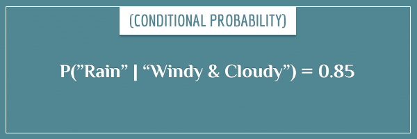
Conditional probabilities expresses the probability that Event-1 will occur when you assume (or know) that Event-2 has already occurred. With this notation, you can write “the probability that it will rain, given that the weather is currently windy and cloudy, is equal to 0.85″ as:

Now let’s ask the following question:

• How does the probability of rain change after finding out the weather is windy and cloudy?

This is precisely the type of question you’d answer with a conditional probability. In the current example, the answer is:

• The probability of rain increased to 0.85.

Remember, we said P(“Rain”) = 0.6. So, you initially thought that rain is moderately likely. Then, after seeing the current weather conditions, you updated your expectations to very likely.

It’s important to clarify that this notation doesn’t imply a causal relationship between the two events. For example, you would also update your expectations for rain after seeing other people carrying umbrellas, even though umbrellas themselves don’t cause rain.

In the current example, you somehow knew that P(Event-1 | Event-2) = 0.85. But is there a way of calculating such probabilities for any kind of events?

How Bayes’ theorem connects probabilities and conditional probabilities

In mathematics, true statements are called theorems. These are statements whose truth you can prove using logic. The proof requires starting from a few basic statements, called axioms.

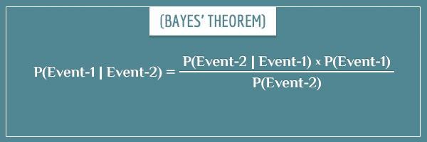
Bayes’ theorem is named after the British statistician and philosopher Thomas Bayes who first discovered it. Let’s look at the mathematical statement it makes:

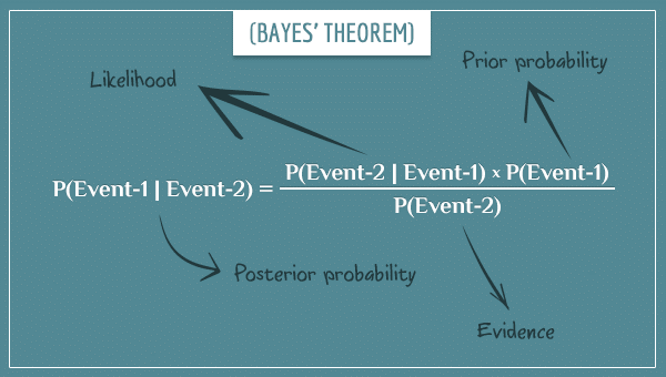
Instead of using concrete event names (like “Rain”), I gave the two events in the equation the general names Event-1 and Event-2. The equation consists of four parts and here’s the traditional terminology for each term:

• P(Event-1): Prior probability
• P(Event-2): Evidence
• P(Event-2 | Event-1): Likelihood
• P(Event-1 | Event-2): Posterior probability

In words, Bayes’ theorem asserts that:

• The posterior probability of Event-1, given Event-2, is the product of the likelihood and the prior probability terms, divided by the evidence term.

In other words, you can use the corresponding values of the three terms on the right-hand side to get the posterior probability of an event, given another event.

By the way, this terminology is traditional Bayesian lingo and you shouldn’t take it too literally. For example, in everyday life, people often use the words “probability” and “likelihood” interchangeably. However, in probability theory, these terms have distinct and specific meanings.

Prior probability

The prior probability of an event (often simply called the prior) is its probability obtained from some prior information.

The word prior can be somewhat misleading. It’s not immediately clear what the probability is prior to. You can think of it as the probability of the event from all the information that is already known. In the weather example, the prior probability of rain was P(“Rain”) = 0.6. This could come (for instance) from the prior knowledge that 60% of the days on the same date have been rainy for the past 100 years.

Here is another way to look at it. A prior probability is always prior with respect to some piece of information that you left out from the calculations. In this example, the information left out when calculating P(“Rain”) = 0.6 is basically everything, except for the past rain frequency for the current date.

Evidence

You started with the prior P(“Rain”) = 0.6 but now you have new information you can use to more accurately estimate the same probability. The evidence term in Bayes’ theorem refers to the overall probability of this new piece of information.

In the current example, we used current weather conditions for updating P(“Rain”), so the evidence would be P(“Windy & Cloudy”). That is, the probability of having windy and cloudy weather, regardless of whether the day turns out to be rainy. You can think of it as the average probability of one event across all possibilities for the other events.

Notice that, outside Bayesian tradition, the word “evidence” is most commonly used to refer to the piece of information itself, and not to its probability. This is a good reminder to not be too literal about these terms.

Likelihood

Unlike the previous two terms, the likelihood represents a conditional probability. In the weather example, this is the probability of having a windy and cloudy morning, given that it ends up raining at least once throughout that day:

   

An intuitive way of thinking about it is the degree to which the first event is consistent with the second event. That is, the above likelihood represents how strongly you expect that the morning will be windy and cloudy if the day ends up being rainy.

Posterior probability

The posterior probability (often just called the posterior) is the conditional probability you’re after when using Bayes’ theorem. It represents the updated prior probability after taking into account some new piece of information. As prior probability is always relative, so is the posterior probability of an event. What this means is that the posterior probability becomes the new prior probability which you can later update again using some other piece of information. And the cycle goes on.

As Dennis Lindley put it:

Today’s posterior is tomorrow’s prior.

In the weather example, the posterior probability was P(“Rain” | “Windy & Cloudy”).

Putting it all together

Now I’m going to take some actual values and use Bayes’ theorem to calculate the posterior probability in our weather example.

The value of the prior probability was already specified to be P(“Rain”) = 0.6. And here are the values for the likelihood and evidence terms:

   

   

The result of plugging in these numbers into the equation is:

   

And yes, I did come up with these numbers so they can nicely fit intо the equation, in order to get the posterior probability P(“Rain” | “Windy & Cloudy”) = 0.85.

Summary

Bayes’ theorem is the mathematical device you use for updating probabilities in light of new knowledge. No other method is better at this job.

Its simplicity might give the false impression that actually applying it to real-world problems is always straightforward. However, getting the correct values of the terms on the right-hand side of the equation can be a challenge. In particular, calculating the evidence term for more complicated problems is often difficult. It might require the use of special mathematical techniques not directly related to the analysis.

Having said that, mathematicians develop and apply new powerful Bayesian algorithms in a wide variety of fields. Some examples include data analysis, artificial intelligence, neuroimaging, forensics, and so on. In future posts, I’m going to discuss those applications which are far more interesting and important than the toy weather example I used here. For a few more concrete examples of its real-world usage in making inferences, check out this post.

Although the post barely scratched the surface of this topic, I hope it gives you a good idea about what makes Bayes’ theorem so exciting. 

---

If you found this topic intriguing, you will probably also like my post Bayes’ Theorem: An Informal Derivation. There, I look at the theorem from a more intuitive point of view and also show its mathematical derivation.

Also, check out my two-part post on Bayesian belief networks to see a really cool way to use Bayes’ theorem for making inferences about multiple events that depend on each other.