In the first part of this post, I gave the basic intuition behind Bayesian belief networks (or just Bayesian networks) — what they are, what they’re used for, and how information is exchanged between their nodes.
In this post, I’m going to show the math underlying everything I talked about in the previous one. It’s going to be a bit more technical, but I’m going to try to give the intuition behind the relevant equations.
If you stick to the end, I promise you’ll get a much deeper understanding of Bayesian networks. To the point of actually being able to use them for real-world calculations.
First, I’m going to start with a recap of what I talked about in the previous post. Then, I’m going to show how to mathematically represent Bayesian networks and make inferences about the states of its nodes.
Reading two of my previous posts would be very helpful along the way, especially if you’re new to the topic.
In the Calculating Compound Event Probabilities post (specifically, the “General formulas for compound events” section) you’ll find the derivation of the formula for the joint probability distribution of multiple events (which I’m going to use here).
Secondly, the post Bayes’ Theorem: An Informal Derivation gives a really good intuition about the way an observation updates the probabilities of rival hypotheses that try to explain it. In particular, I recommend the section explaining the evidence term of Bayes’ theorem because here I’m going to use a very similar method in explaining the math of information propagation in Bayesian networks.
Table of Contents
Bayesian networks
Bayesian networks consist of nodes connected by arrows. You usually graphically illustrate the nodes as circles.
Each node represents the probability distribution of a set of mutually exclusive outcomes. For example, a node can represent the outcome of rolling a die, with each side having a probability of to be on top. Or the outcome of flipping of a coin, with each side having a probability of
.
More generally, each node represents the possible states of a variable and holds their respective probabilities.
The arrows hold the information about the conditional probabilities between the nodes they connect. The node the arrow is pointing to (the child node) depends on the arrow it originates from (the parent node). This means that the probability of a child node taking a particular state will depend on the state of its parent.
States of nodes in the network
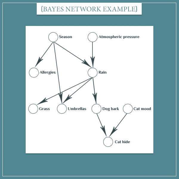
In the first post, I came up with this example for a Bayesian network:
In this example, the “Season” node’s possible states are:
- Spring
- Summer
- Fall
- Winter
Similarly, the “Rain” node’s states are:
- It’s raining
- It’s not raining
You get the idea.
If you haven’t made any observations related to the network, then each node will be in one of its possible states with a certain probability. For example, if you pick a random day of the year (but you haven’t seen the day you’ve picked yet), the probability that you’ve picked any of the 4 possible seasons is (assuming the seasons are of equal length). So, the “Season” node’s probability distribution is:
If you observe the value of a node, its state is no longer probabilistic. For example, if you already know that the day you’ve picked is July 17, the probabilities for the “Season” node become:
This simply reflects the fact that once you’ve observed a node, there’s no longer uncertainty about which state it’s in.
Dependence between states
If there’s an arrow between two nodes, the state of the child node will probabilistically depend on the state of its parent. Hence, you express this as a conditional probability of one node given another:
In other words, this is the probability of Node 2 being in State X, if Node 1 is State Y. For example, if the season is fall, the probability of rain will be higher than if the season is summer:
By the way, this dependence between nodes is precisely what allows information propagation within Bayesian networks. Observing the state of a node updates the probabilities of its children and its parents. Then, the newly updated nodes update their children/parents, and so on.
The state of the whole network
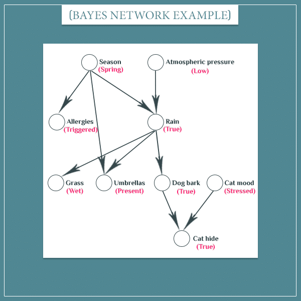
A very useful thing to be able to represent simultaneously is the states of all network nodes. Here’s an example:
You see that each node is now in a particular state, instead of being in a state of uncertainty (the pinkish labels below the node names indicate the current state).
You can think of a set of node states as the state of the whole network. This state is known with certainty if you’ve observed the states of each node in the network.
Consequently, the total number of network states is equal to the number of all combinations of node states (usually a very high number for most networks). Each network state has a probability of its own, which is the joint probability over all node states. And the list of all joint probabilities is the joint probability distribution of the network.
(I’m assuming you’re already familiar with joint probabilities. If not, please take a look at the 2 posts I linked to in the beginning.)
You write the joint probability of the example state above as:
- P(Spring, Low atmospheric pressure, Wet grass, Cat stressed…)
Notice that the expression above specifies the states of the nodes. A more explicit notation would look like:
- P(Season = Spring, Atmospheric pressure = Low, Grass = Wet, Cat mood = Stressed…)
More generally, you can express the joint probability distribution just by writing the names of the nodes:
- P(Season, Atmospheric pressure, Grass, Cat mood…)
The names are simply placeholders and can be replaced by particular states — either hypothetically or if the states are actually observed.
The joint probability distribution of a network
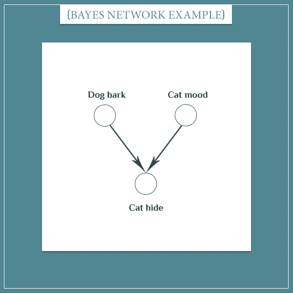
Expanding the joint probability above is done according to this formula. I’m not going to write the full expression here because it is very long. Instead, let’s look at a smaller part of the network:
Then, according to the formula, the joint probability distribution of this small network would be:
- P(Dog bark, Cat mood, Cat hide) = P(Dog bark) * P(Cat mood | Dog bark) * P(Cat hide | Dog bark, Cat mood)
But here’s the beautiful part. The absence of an arrow between nodes means that the nodes are independent (it’s what you’re essentially assuming about 2 nodes if you don’t put an arrow between them). And this allows you to drop the dependency between those nodes in any further calculations.
In this case, there’s no arrow between the “Dog bark” and “Cat mood” nodes, which slightly simplifies the expression on the right-hand side to:
- P(Dog bark, Cat mood, Cat hide) = P(Dog bark) * P(Cat mood) * P(Cat hide | Dog bark, Cat mood)
By not having an arrow between two nodes, you’re basically assuming that the nodes are independent. But in reality they might not be and that would be a flaw of your network.
So, the presence/absence of arrows determines the dependency structure of the network. Once you have that, you also need to define the exact dependencies between the nodes with arrows, as well as the prior probabilities of the nodes without arrows. And you’re done: this defines the entire Bayesian network!
The final expression
Now, with this information in mind, I can actually write the joint distribution of the entire network from the example above, because it’s no longer that long:
- P(Network) = P(Season) * P(Atmospheric pressure) * P(Allergies | Season) * P(Rain | Season, Atmospheric pressure) * P(Grass | Rain) * P(Umbrellas | Season, Rain) * P(Dog bark | Rain) * P(Cat mood) * P(Cat hide | Dog bark, Cat mood)
I’m using the shorthand notation P(Network) to refer to the joint probability distribution over the nodes. And I’m going to use the same notion in the rest of this post.
The conditional probabilities are colored in red and the unconditional (prior) probabilities are colored in green. Notice how each node is only conditioned on its parents. Importantly, this really shortened an expression that would otherwise be extremely long and difficult to read! Hover or click over here to see what I’m talking about.
To sum up, the joint probability distribution of Bayesian networks is simply the product of the probabilities of its nodes. Each probability is conditioned only on the parents of the respective node and nodes that have no parents only have a prior probability.
The full joint probability without taking advantage of the dependency structure of the network
P(Network) = P(Season) * P(Atmospheric pressure | Season) * P(Allergies | Atmospheric pressure, Season) * P(Rain | Season, Atmospheric pressure, Allergies) * P(Grass | Season, Atmospheric pressure, Allergies, Rain) * P(Umbrellas | Season, Atmospheric pressure, Allergies, Rain, Grass) * P(Dog bark | Season, Atmospheric pressure, Allergies, Rain, Grass, Umbrellas) * P(Cat mood | Season, Atmospheric pressure, Allergies, Rain, Grass, Umbrellas, Dog bark) * P(Cat hide | Season, Atmospheric pressure, Allergies, Rain, Grass, Umbrellas, Dog bark, Cat mood)
Making inferences about the states of nodes
So, we finally come to the interesting part. Imagine you have a network with a specific joint probability distribution P(Network). As you already know, if the state of one node is observed, this is going to change the probabilities of the states of (some) other nodes in the network.
In this section, I’m going to show how to mathematically calculate these new probabilities, called posterior probabilities,.
Conditioning the joint distribution on observations
Before any node is observed, each will have a particular prior probability distribution over its states. Then, if a particular node’s state is observed, its probability distribution is changed to 1 for the observed state and 0 for the other states.
Subsequently, the posterior probability distribution of the remaining nodes is calculated according to Bayes’ theorem:
You’ll remember this particular representation of Bayes’ theorem from my post Bayes’ Theorem: An Informal Derivation I linked to in the beginning. More specifically, from the “More intuition about the evidence” section.
So, you see that all it takes to calculate the joint posterior distribution of the network is to divide its joint prior distribution by the marginal probability of the observed node. Yes, it’s really that simple!
Similarly, if you’ve observed the states of multiple nodes, you simply condition the full joint distribution on all observed nodes. This means that, on the right-hand side of the equation you will divide by the joint distribution of the observed nodes.
The intuition behind conditioning on observed states
For this section, I’m going to borrow an example from the post I linked to above.
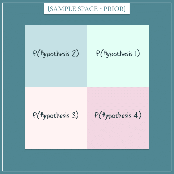
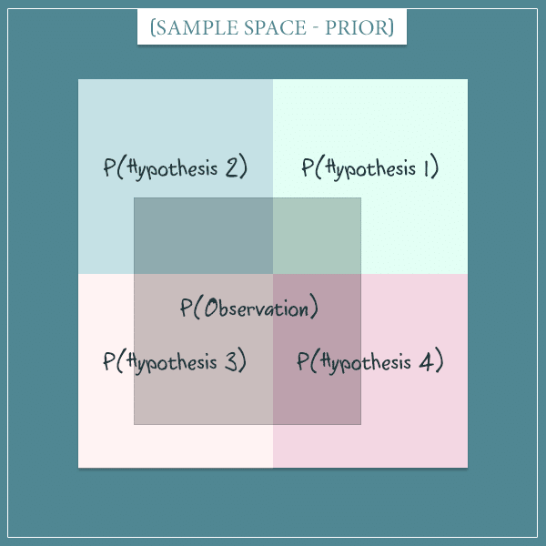
Imagine there are 4 mutually exclusive hypotheses that attempt to explain something general about the world. Further, assume that in the beginning each hypothesis is equally likely. Here’s a visual representation of the sample space of this hypothetical world:
Each of the 4 squares represents one of the hypotheses and all squares have the same area (because we said they have equal prior probabilities). So, each hypothesis has a probability of .
Now, imagine that you learn something about the world by making an observation of some of its states. Moreover, let’s say the new observation covers a specific part of the sample space:
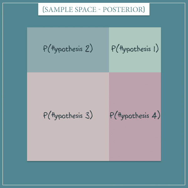
The dark square represents the probability of the observation you just made (the probability it had before you made it, actually). And now that you’ve made the observation, you can exclude all the states outside of it. This simply means that the dark square becomes your new sample space:
In other words, you now know that part of the sample space is actually the world you’re living in: namely, the only parts of the old sample space that are consistent with the observation.
This new sample space represents the posterior probability distribution over the 4 hypotheses. Notice how their probabilities have changed and they’re no longer equally probable. This is because some of them were more consistent with the observation than others.
This may still sound a little abstract, but I just wanted to give a quick reminder of how you update probabilities with Bayes’ theorem after new observations. In the next section, I’m going to show an application to a specific example that should make everything I’ve talked about so far much clearer.
Example
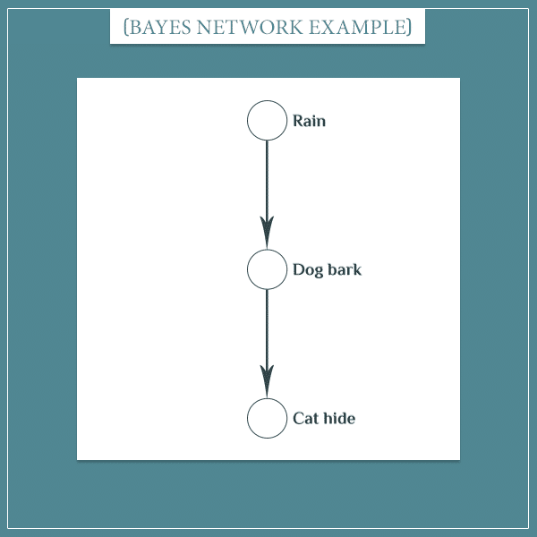
So, let’s consider a small part of the Bayesian network I’ve been working with so far:
This was actually the very first example I gave in the previous post. In short, when it rains, the dog tends to bark at the window. And when the dog barks, the cat tends to hide under the couch.
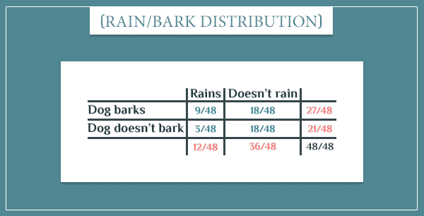
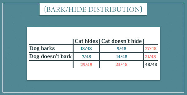
Next, let’s consider only the top two nodes. The specific probability distribution for the “Rain” and “Dog bark” nodes I came up with last time was:
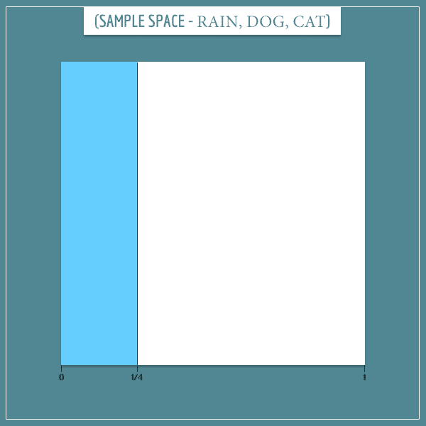
Okay, let’s start building the sample space. First of all, there is a probability that it rains and
probability that it doesn’t rain:
Notice how the blue area (representing rain) covers of the sample space.
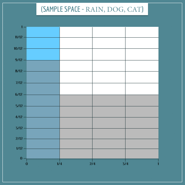
Now, let’s superimpose the sample space of the “Dog bark” node onto the sample space of the “Rain” node:
Notice how 9 out of 12 “Rain” rectangles are also gray. This corresponds to the top left cell in the probability table above:
Similarly, 18 out of the 36 “No rain” rectangles are gray, which corresponds to the probability:
In the same manner, you can calculate the remaining probabilities from the table.
Okay, what about the “Cat hide” node? Its probability table was:
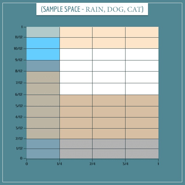
Can we similarly superimpose it on the same sample space? Absolutely!
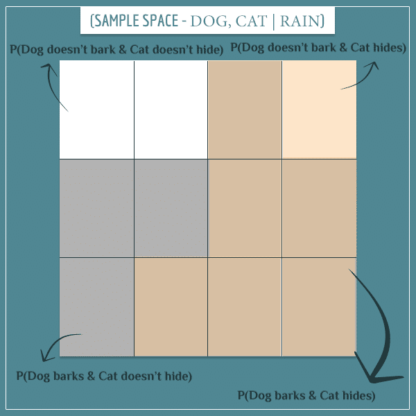
Importantly, notice the beige colored rectangles representing the “Cat hides = True” event. I’ve carefully colored all rectangles so that this 3-way joint sample space doesn’t contradict any of the probability tables.
Making inferences
Now imagine you’ve actually looked at the weather outside and you know it’s currently raining. Then, you calculate the new (posterior) joint distribution of the network by conditioning it on the “Rains” event:
Expanding the right-hand side of the equation, we get:
The P(Rains) terms cancel out and the final posterior distribution becomes:
So, what does the posterior sample space look like? Remember, because we know it’s currently raining, we ignore the parts of the sample space representing the “Doesn’t rain” event. Therefore, we only take the 12 blue rectangles on the left and make them the new sample space:
Can you see which of these 12 rectangles corresponds to which of the 12 rectangles from the left-most column from the prior sample space?
Out of these 12 rectangles:
- 3 represent the “Dog barks & Cat doesn’t hide” event
- 6 represent the “Dog barks & Cat hides” event
- 2 represent the “Dog doesn’t bark & Cat doesn’t hide” event
- 1 represents the “Dog doesn’t bark & Cat hides” event
Now we can answer all sorts of probabilistic questions about the individual events. For example, there are 9 “Dog barks” rectangles in total, which means the posterior probability of the dog barking is:
Remember, the prior probability P(Dog barks) was .
Similarly, there are 7 “Cat hides” rectangles, so the posterior probability of this event is:
Which is also higher than the prior .
The big picture
To summarize, in order to calculate the posterior probability distribution of Bayesian networks, you divide the prior probability distribution by the probability of the observed event(s). The theory is as simple as that.
I tried to give the intuition behind this calculation by visually showing how the sample space changes after a particular observation. But you obviously don’t have to draw sample spaces every time you want to update the probability distribution of a Bayesian network. In practice, you just apply the formula.
The mathematical expression for the example above was:
Take another look at the prior sample space:
Again, 9 out of the 12 “Rain” rectangles are also gray (which represent the “Dog barks” event.) This means:
Similarly, 18 out of the 27 “Dog barks” rectangles are also colored in beige (which represents the “Cat hides” event). Therefore:
Therefore, the final expression for P(Dog barks, Cat hides | Rains) becomes:
If you go back to the posterior sample space, you’ll notice the “Dog barks & Cat hides” compound event is represented by exactly 6 out of 12 rectangles:
As expected, the result is the same!
And a specific event’s posterior probability would be equal to its posterior marginal probability.
In practice, things aren’t always as smooth. For more complex networks, calculating the evidence term or the marginal probability of individual events can be a mathematical challenge. These cases are topics for future posts.
Summary
In this post, I gave the mathematical intuition behind Bayesian networks which I had introduced in Part 1.
To sum up, whether you’re making future predictions or inferences about possible explanations of observations, all you need to do to calculate the posterior distribution of the network is to condition it on the observed nodes. Which simply means to divide the prior joint probability distribution of the network by the joint probability of the observed states.
As I mentioned at the end of the last section, in practice many Bayesian belief networks are too complex and there is no exact mathematical solution for their posterior distributions. In such cases, people use different numerical methods to get an approximate solution. Because these are relatively advanced topics, I plan to cover them in future posts. But you don’t have to worry about them for now. If you feel comfortable with the concepts and methods I introduced in these two posts, you will be able to build simple networks and calculate probabilities with them. And if you have a programming background, you will probably even be able to write your own simple networks to make calculations faster.
In some of my next posts, I’m going to show applications of Bayesian belief networks to some real-world problems. I think this will give even better intuition on how useful this tool really is.
One topic that I wanted to cover in this post, but didn’t, was the concept of conditional dependence and independence between nodes. In short, two nodes that were otherwise dependent can become independent if a particular third node’s state is observed. Similarly, nodes that were otherwise independent can become dependent, again after observing a particular third node.
Check out my next post if you’d like to learn more about this topic!



HI,
not sure I got it
P(Dog barks, Cat hides | Rains) = P(Cat hides | Dog barks) * P(Dog barks | Rains)
I thought the 1st term on right hand side is P(Cat hides | Dog barks, Rain)
Hi Haibin, good question!
In fact you are right, the full expression P(Dog bark, Cat hide | Rain) is equal to looks like this:
Simplified (when you cancel the P(Rain) terms):
On the other hand, you have:
This is from exploiting the dependency structure of the nodes in the graph, as explained in the sub-section The joint probability distribution of a network.
Hence, you finally get:
P(Dog barks, Cat hides | Rains) = P(Cat hides | Dog barks) * P(Dog barks | Rains)
Does that clarify things?
in the section ‘Conditioning the joint distribution on observations’
is there a typo in the formula box ‘Baye’s theorem’ ?
P(network | node-x) = P(network) / P(node-x)
shouldn’t it be :
P(network | node-x) = P(network, node-x) / P(node-x)
Hey, Noel!
If a network consists of nodes {a, b, c}, the expression P(network) is equivalent to P(a, b, c). In other words, in the example you cited, P(network) already includes node-x, so there is no need to write it again.
Still, could you share your reasoning for why you thought it should be P(network | node-x) = P(network, node-x) / P(node-x)? Maybe I can help you clarify something else that you’re not sure you understood completely.
By the way, to get a little more intuition about this, just imagine the simplest possible network consisting of only 2 nodes: node-x and node-y. Then you would have:
(1)
Another way to express the joint probability on the right-hand side is:
(2)
Are you with me so far?
Also assume that each node only has 2 states: 0 and 1. The probability of a particular state of the network (say, that both nodes are in state 1) could be written as:
(3)
Now imagine you’ve observed that node-x is actually in state 1 and you want to calculate the probability that node-y is also in state 1. Then according to the equation P(network | node-x) = P(network) / P(node-x) and the 3 equations above, this would be given by:
(4)
Which is equal to:
(5)
Note that for the left-hand side of equation 4 we have P(network | node-x=1) = P(node-x=1, node-y=1 | node-x=1) = P(node-y=1 | node-x=1) (do you agree?). Then we finally get that P(node-y=1 | node-x=1) is equal to:
Or, more generally:
Which is simply Bayes’ theorem.
Please let me know if this answers your question.
Hi
Thank you for the thorough expalanation regarding the topic. I have a question regarding the joint probability distribution of the entire network:
P(Network) = P(Season) * P(Atmospheric pressure) * P(Allergies | Season) * P(Rain | Season, Atmospheric pressure) * P(Grass | Rain) * P(Umbrellas | Season, Rain) * P(Dog bark | Rain) * P(Cat mood) * P(Cat hide | Dog bark, Cat mood)
about the term P(Umbrellas | Season, Rain). Since umbrellas and season are independent, won’t it be just P(Umbrellas | Rain)?
Hi, Ridzky!
The Umbrellas and Season variables (nodes) aren’t independent. You see that there’s an arrow from Season to Umbrellas, right? This means that P(Umbrellas | Season) is not equal to P(Umbrellas).
You might be wondering why that’s the case. If there’s no rain, why would the season change the probability of people carrying umbrellas? Well, the basic intuition here is that some people are more likely to carry umbrellas during rainy seasons, even if it’s not raining on a particular day. Maybe they haven’t checked the weather forecast or they’re trying to be prepared in case the forecast happens to be wrong.
In other words, the fact that the distribution of the Umbrellas node is P(Umbrellas | Season, Rain) and not P(Umbrellas | Rain) implies statements like:
It’s more likely to see people with umbrellas during rainy seasons than during dry seasons. And even more likely if it’s a rainy season and it’s actually raining.
Does this make sense?
Thank you for quick response. I didn’t realize that both umbrellas node and season node are connected. At first, I just thought that they weren’t connected. Thanks again for the answer!
Hey,
How can I expand this: P(HD=yes|BP=high, D=Healthy, E=yes) = ?
Hi Ahmed,
Without any information regarding the joint probabilities, you can only write it as (using the general Bayes’ theorem formula):
But, depending on the type of Bayesian network that would adequately represent these 4 variables, you could construct a simpler expression on the right-hand side, as I explained in the second half of the post. Let me know if anything in those sections is difficult to understand and I can help you with the details.
P(Dog barks, Cat hides | Rains) = P(Cat hides | Dog barks) * P(Dog barks | Rains)
I was looking for an explanation of the above equation from some other notes and I am glad you have explained this clearly to someone else promptly.
Very good