Bayes’ Theorem: An Informal Derivation

If you’re reading this post, I’ll assume you are familiar with Bayes’ theorem. If not, take a look at my introductory post on the topic.

Here I’m going to explore the intuitive origins of the theorem. I’m sure that after reading this post you’ll have a good feeling for where the theorem comes from. I’m also sure you will find the simplicity of its mathematical derivation impressive. For that, some familiarity with sample spaces (which I discussed in this post) would come in handy.

So, what does Bayes’ theorem state again?

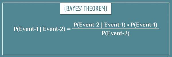
Here’s a quick reminder on the terms of the equation:

• P(Event-1): Prior probability
• P(Event-2): Evidence
• P(Event-2 | Event-1): Likelihood
• P(Event-1 | Event-2): Posterior probability

Put simply, Bayes’ theorem is used for updating prior probabilities into posterior probabilities after considering some piece of new information (that is, some piece of evidence). The exact way the updating process takes place is given by the relationship asserted by the theorem. Namely, the posterior probability is obtained after multiplying the prior probability by the likelihood and then dividing by the evidence.

But have you wondered where this exact relationship comes from? The easiest way to answer the question is by first defining joint probabilities and showing how the theorem naturally pops out.

Joint probabilities and joint sample spaces in the context of Bayes’ theorem

The joint probability of two events is simply the probability that the two events will both occur. The most common mathematical notation for expressing a joint probability is:

   

Notice the difference with the notation for conditional probabilities where there is a vertical line between the two events (instead of a comma).

Imagine you’re simultaneously flipping a coin and rolling a die. A joint probability example would be the probability of flipping heads and rolling an even number in a single repetition:

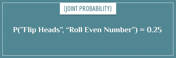
You can get to this probability from a graphical analysis of the sample space. As a reminder, the sample space of a random process is the set of all possible outcomes of that process. The joint sample space of two random processes is all possible combinations of outcomes of the two processes. Take a look:

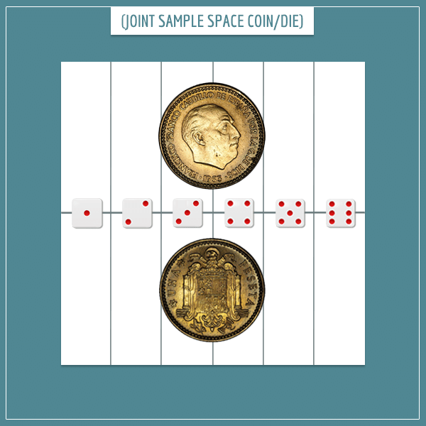
The horizontal line divides the square into 2 equal parts which represent the outcome of the coin flip.

The vertical lines further divide the square into 6 equal parts which represent the possible outcomes of rolling the die. You see that when the two sample spaces are superimposed on each other the square is divided into 12 equal rectangles. Each rectangle represents а possible combination, like:

• “Flip Heads”, “Roll 1”
• “Roll 4”, “Flip Heads”
• “Flip Tails”, “Roll 3”
• Etc.

The marked rectangles in the image below represent the event of flipping heads and rolling an even number:

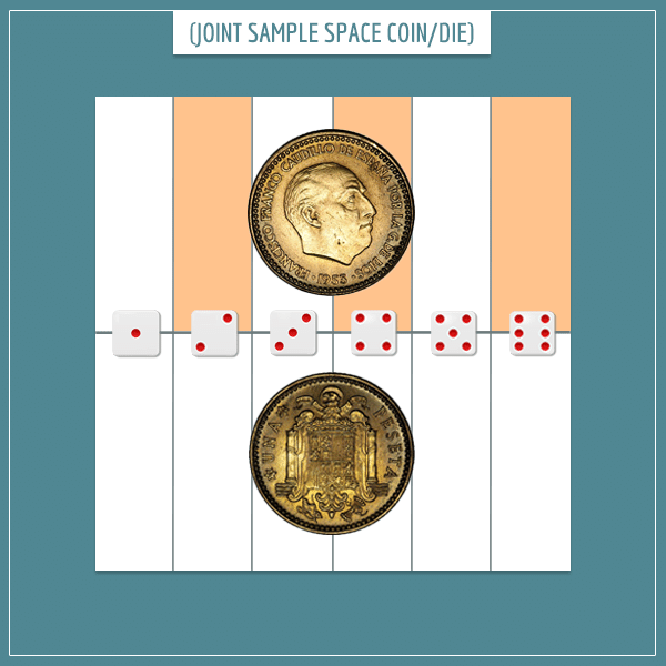
First, the rectangles are from the upper half of the square which stand for the probability of flipping heads. Second, only those rectangles associated with rolling one of the three even numbers are marked. As you can see, 3 out of the 12 (or 1/4) of the rectangles satisfy the definition of the event.

The sum of the areas of the marked rectangles is the area of the intersection of the two events. You can calculate the joint probability by considering the fraction of the total area that it covers:

   

An alternative look at joint probabilities

Here’s a very important relationship between probabilities, conditional probabilities, and joint probabilities:

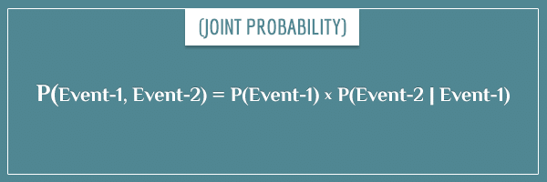
The joint probability of two events is the probability of the first event times the conditional probability of the second event, given the first event. Why? This part is slightly tricky, so arm yourself with your abstract reasoning skills.

Remember, the joint probability of two events is the probability that both events will occur. For that, first one of the events needs to occur, which happens with probability P(Event-1).

Then, once you know Event-1 has occurred, what is the probability that Event-2 will also occur? Naturally, this is the conditional probability P(Event-2 | Event-1): the probability of Event-2, given Event-1.

Тhe conditional probability is simply the fraction of the probability of Event-1 which also allows Event-2 to occur. In other words, to get the joint probability of two events, you need to take the fraction of P(Event-1) that is consistent with the occurrence of Event-2. To take the fraction of something really means to multiply that “something” by the fraction:

   

The joint probability from the previous example becomes:

   

You can infer the values of the two terms on the right-hand side from the joint sample space:

   

   

Then:

   

The result is the same as with the previous approach. Pretty neat.

The incredibly simple derivation of Bayes’ theorem

Now that you’ve convinced yourself about the last relationship, let’s get down to business.

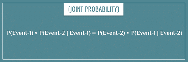
First, notice that the relationship can be stated in two equivalent ways:

   

   

The intuition behind this symmetry is that the order of the events isn’t a concern. You only care about their intersection in the sample space, which is the probability of both events occurring (for more intuition on this, check out my post about compound event probabilities).

However, that doesn’t mean the terms are in any way interchangeable in general. Each term represents a different subset of the sample space and hence a different probability or conditional probability. However, if you combine the two equations, you can see that the expressions on the right-hand side are really equal to the same thing. And, therefore, they are equal to each other:

To get to Bayes’ theorem from here, you only have to divide both sides of the equation by P(Event-1) or P(Event-2):

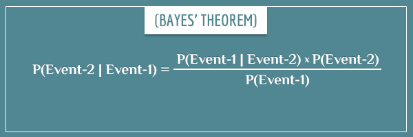
Yes, this is really it. Now you officially know the origin of Bayes’ theorem! I told you it was simple.

Okay, this is one way to mathematically derive it. It’s still not quite enough to get a good feeling for it, however. Does Bayes’ theorem make intuitive sense or is it some mathematical truth that you just have to accept? I’m dedicating the final section of this post to exploring this question.

The intuition behind the theorem

Imagine you have a hypothesis about some phenomenon in the world. What is the probability that the hypothesis is true?

To answer the question, you make observations related to the hypothesis and use Bayes’ theorem to update its probability. The hypothesis has some prior probability which is based on past knowledge (previous observations). To update it with a new observation, you multiply the prior probability by the respective likelihood term and then divide by the evidence term. The updated prior probability is called the posterior probability.

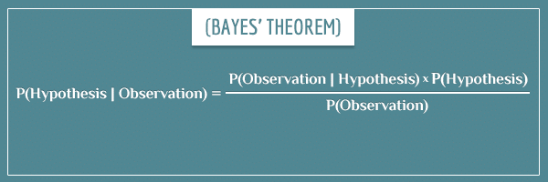
The posterior probability then becomes the next prior which you can update from another observation. And so the cycle continues.

Notice the dependence between the posterior probability and the three terms on the right-hand side of the equation. All else being equal:

1. A large prior probability term will make the posterior probability larger (compared to a small prior probability).
2. Similarly, a large likelihood term will make the posterior probability larger.
3. A large evidence term will make the posterior probability smaller.

These relationships come from the fact that the posterior is directly proportional to the prior and likelihood terms, but inversely proportional to the evidence term.

Now, the first relationship should be pretty intuitive. All else being equal, the posterior probability will be higher if you already had strong reasons to believe the hypothesis is true. But what about the other two relationships?

Let’s explore this in some more detail.

The likelihood

The likelihood reads as “the probability of the observation, given that the hypothesis is true”.

This term basically represents how strongly the hypothesis predicts the observation. If the observation is very consistent with your hypothesis, all else being equal, it will increase the posterior probability.

Similarly, if according to your hypothesis the observation is very unlikely and surprising, that will reduce the posterior probability.

Here’s a simple example that makes this intuition explicit.

Say someone tells you that there’s some living being on the street: I’ll name it Creature. Your strongest hypothesis is that Creature is a human (because of the frequency with which you’re used to seeing humans in your neighborhood, compared to other animals). That is, the prior probability P(Human) is high.

Next, you have the following observation:

• Creature is wearing clothes.

Now the posterior probability (the “new prior”)  is:

   

The corresponding likelihood term is:

   

The value of this likelihood will obviously be very high. It’s not that it’s impossible to come across a naked person on the street, but the probability is quite low.

On the other hand, if you know that Creature is currently barking, the following likelihood term will have a very low value:

   

To sum up, the more consistent the observation is with the hypothesis, the more probable it is that the hypothesis is true. This aspect of Bayes’ theorem should also have a strong intuitive appeal.

The evidence

In the context of Bayes’ theorem, the evidence is the probability of the observation used to update the prior. Examples of such observations are:

• Creature has 4 legs
• It is breathing
• It is inside a car

I’ll change the example a little bit and say there are only 4 equiprobable hypotheses about Creature:

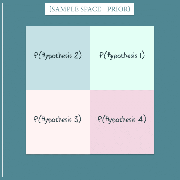
The four hypotheses can, for example, represent “human”, “dog”, “cat”, and “mouse”.

The uncertainty is currently too high and you decide to collect more information to update the probabilities. You’re hoping to make some observations about Creature to help you narrow down the posterior and make it somewhat more informative.

The effect of the evidence on the sample space

Let’s say you make a particular observation. After you make it, you can represent the probability it had prior to making it in the same sample space like so:

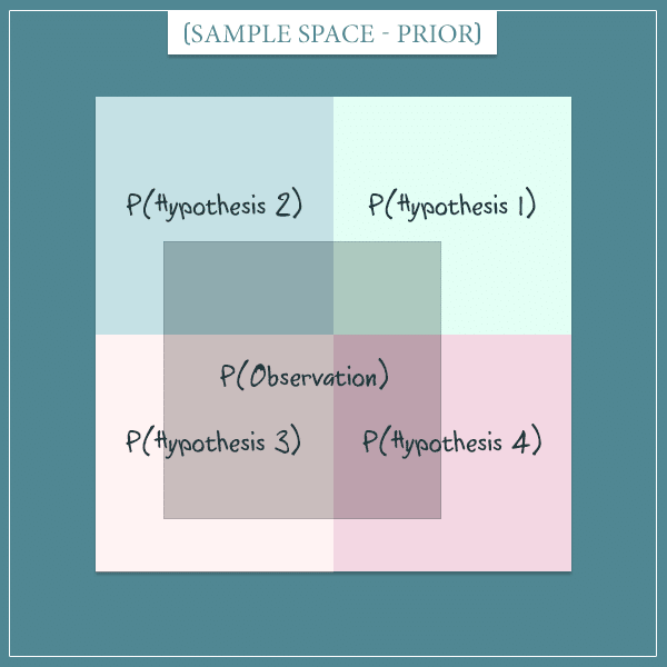
Think about the sample space as representing all possible worlds. Some of those worlds are consistent with the observation and are bound within the dark square depicting P(Observation).

Now this is the crucial part. The above is the old sample space. After you make the observation, you eliminate the worlds that are inconsistent with the observation from the sample space.

For example, if you learn that Creature has 4 legs, you will ignore the worlds in which Creature has any different number of legs. Those worlds would be the parts of the sample space outside P(Observation). In other words, the world you live in happens to be within the area of P(Observation).

Therefore, that area now becomes the new sample space:

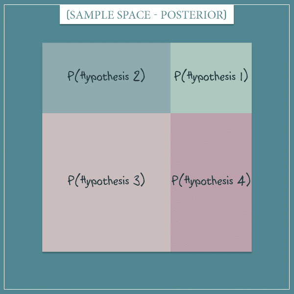
Remember that the total probability of a sample space is always equal to 1. So, you redistribute this probability among the hypotheses proportionally to the percentage of the new sample space they occupy.

Each hypothesis used to have a probability of 0.25 but this is no longer the case. For example, you can see that in the updated sample space Hypothesis 3 has gained a much larger portion, whereas Hypothesis 1’s probability has shrunk significantly. That is because Hypothesis 3 covers a larger portion of P(Observation).

Well, this is Bayes’ theorem in a nutshell! The “old” sample space represents the prior probability and the “new” sample space represents the posterior probability of each hypothesis.

More intuition about the evidence

Take another look at the second-to-last image above. Before you make the observation, the overlap between the area of P(Observation) and the area of a particular hypothesis is actually their joint probability. Notice that the 4 joint probabilities completely cover P(Observation). You can express this as their sum:

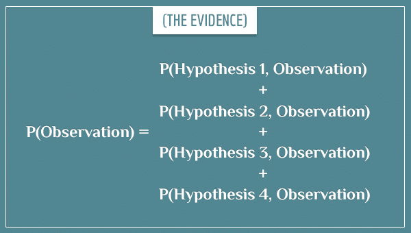
Remember that the numerator in Bayes’ theorem is one of those joint probabilities. The denominator is the evidence: as I just showed, it’s also the sum of all joint probabilities. So, the posterior probability P(Hypothesis | Observation) is the fraction of the area of P(Observation) covered by P(Hypothesis, Observation):

   

You can think about it as the portion of the observation that your hypothesis explains (in relation to how much the other hypotheses explain it).

Since the evidence term is in the denominator, it’s inversely proportional to the posterior probability. That is, the higher the evidence, the lower the posterior is going to be.

To understand this, think about what makes the evidence term grow in the first place.

If P(Observation) is high, that means the observation wasn’t a surprising one and it was probably strongly predicted not just by your hypothesis, but by some of the alternative hypotheses. For example, if your observation is that Creature is breathing, the posterior P(Creature is a human | Creature breathes) won’t be too different from the prior P(Creature is a human). The reason is that, even though this observation is consistent with the hypothesis, it is equally consistent with all alternative hypotheses and it will support them just as much.

On the other hand, if P(Observation) is small, that means the observation was surprising and unexpected. A hypothesis which happens to strongly predict such an observation is going to get the largest boost of its probability (at the expense of the probabilities of the other hypotheses, of course).

Summary

In this post I presented an intuitive derivation of Bayes’ theorem. This means that now you know why the rule for updating probabilities from evidence is what it is and you don’t have to take any part of it for granted. I also gave some insight on the relationship between the 4 terms of the equation.

Perhaps you already understood the theorem, but now you also feel it! So, go ahead and start confidently applying it in whatever areas interest you most.

---

To get more experience and even more intuition about Bayes’ theorem, check out my posts on Bayesian belief networks and applying Bayes’ theorem to solving the so-called inverse problem.