In this post, I want to talk about conditional dependence and independence between events. This is an important concept in probability theory and a central concept for graphical models.
In my two-part post on Bayesian belief networks, I introduced an important type of graphical models. You can read Part 1 and Part 2 by following these links.
This is actually an informal continuation of the two Bayesian networks posts. Even though I initially wanted to include it at the end of Part 2, I decided it’s an important enough topic that deserves its own space.
If you already feel comfortable with Bayesian networks, you shouldn’t have any problems understanding conditional dependence and independence.
Table of Contents
How can events depend on each other conditionally?
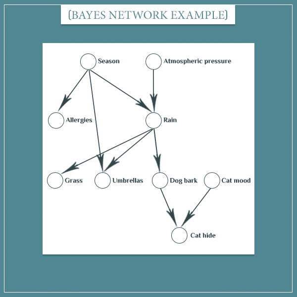
Remember that Bayesian networks are all about conditional probabilities. Each node of the network has a probability distribution over its possible states. Nodes connected with arrows are dependent in the sense that information about one node changes the probability distribution of the other.
There’s a simple example I keep using to illustrate conditional probabilities. If you know that there are dark clouds in the sky, the probability that it will rain will increase. And the other way around: sunny weather would make rain less likely.
On the other hand, nodes not connected with arrows are independent.
However, even if there is no arrow between two nodes, they can still depend on each other. This is because, as you know, information from one node can travel upwards to its parents and downwards to its children.
More interesting cases arise when two nodes that were otherwise dependent become independent when there’s information about a third node’s state. The opposite can also occur and two independent nodes can become dependent, given a third node.
I’m going to show how each of the two works in the rest of this section.
Conditional independence
In the Bayesian network posts, I came up with an example with which I showed how information propagates within the network.
Feel free to read more details about this network.
For the first example of conditional independence, I’m going to take a small part of the network.
![]()
As a reminder, the situation here is that there’s a dog that likes barking at the window when it’s raining outside. There’s also a cat that tends to hide under the couch when the dog is barking for any reason.
Translated to the language of probability, the two sentences above become:
![\[ P(\textrm{Dog barks} \mathbin{\vert} \textrm{Rains}) > P(\textrm{Dog barks}) \]](https://www.probabilisticworld.com/wp-content/ql-cache/quicklatex.com-22347082e4ad48f5789d73be676cd61b_l3.png "Rendered by QuickLaTeX.com")
![\[ P(\textrm{Cat hides} \mathbin{\vert} \textrm{Dog barks}) > P(\textrm{Cat hides}) \]](https://www.probabilisticworld.com/wp-content/ql-cache/quicklatex.com-6072c0ad6183d7de223e6c55be028e49_l3.png "Rendered by QuickLaTeX.com")
Even though there’s a direct connection between the “Rain” and “Cat hide” nodes, they’re not independent. If you know that it’s currently raining, then you’ll know it’s more likely that the dog is barking. That, in turn, will make it more likely that the cat is hiding under the couch.
Similarly, if you know that the cat is hiding, the probability that the dog is barking will also increase. The reason is that the dog’s barking is one of the possible things that can make the cat hide. For the same reason, knowing that the dog is more likely to be barking will increase the probability that it’s currently raining.
But think about what happens in the same situation if you already know the dog is barking. Will observing rain still increase the probability that the cat is hiding under the couch? The answer is no.
The “Rain” node was able to influence the “Cat hide” node only to the extent that it was influencing the “Dog bark” node. However, if we already know the state of “Dog bark”, this will fix its probability at 1.
The mathematical intuition
The consequence of the “Dog bark” node’s state being fixed is that you can no longer update it.
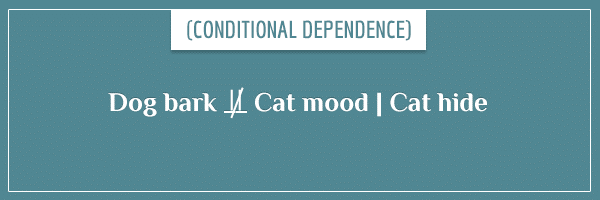
Basically, if a node is observed, it blocks the information propagation that would have otherwise “passed” through it. In the current example, we say that the “Rain” and “Cat hide” nodes are conditionally independent, given the “Dog bark” node. Here’s the mathematical notation that expresses this:
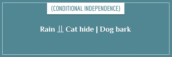
The symbol between “Rain” and “Cat hide” means “are conditionally independent”. The vertical line that separates “Dog bark” is the usual notation for conditional probabilities.
So, the whole expression reads as:
- The “Rain” and “Cat hide” nodes are conditionally independent, given the “Dog bark” node.
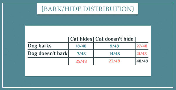
Okay, let’s prove that this conditional independence really holds. The two dependencies from the graph above are:
- “Dog bark” | “Rain”
- “Cat hide” | “Dog bark”
And here are their probability tables:
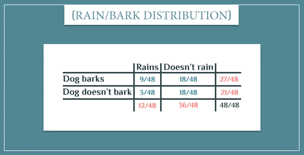
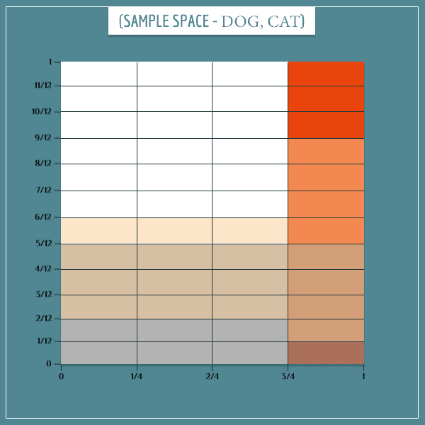
Now, let’s look at the sample space of this graph (click here to see more details about its construction):
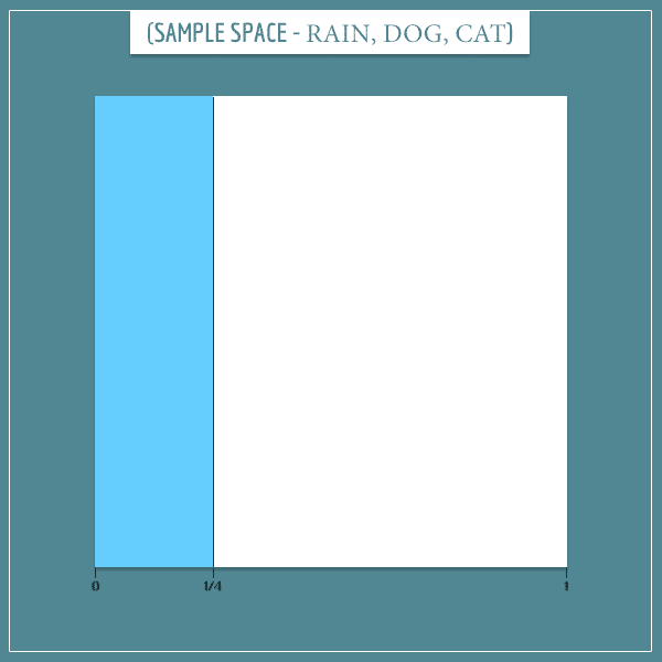
This part simply captures the 1/4 probability of rain. We still need to add the “Dog bark” and “Cat hide” node information. Here’s the first:
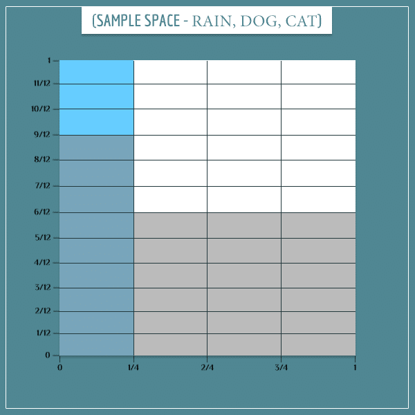
Notice how the gray rectangles are unevenly distributed over the blue and white parts of the sample space. This simply captures the information that the dog is more likely to bark if it’s raining compared to if it’s not raining (compare this sample space to the first probability table above).
Finally, we add the “Cat hide” node to the sample space:
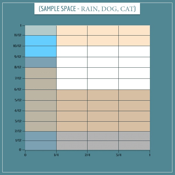
Again, notice how the distribution of beige rectangles over the gray and white rectangles isn’t even. This captures the information that the cat is more likely to be hiding if the dog is barking. And, because the dog is more likely to be barking if it’s raining, it indirectly captures the information that the cat is also more likely to be hiding if it’s raining.
Conditioning on the connecting node
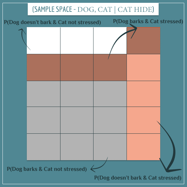
Now, check what happens if we’ve observed that the dog is barking:
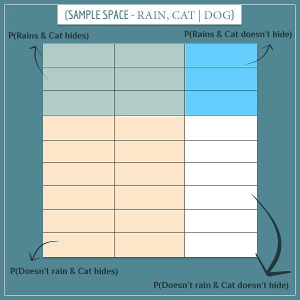
The new sample space consists only of the 27 gray rectangles corresponding to the “Dog barks” event.
Basically, the top left and top right rectangles represent the “Rains” event and the bottom left and bottom right (in white) represent the “Doesn’t rain” event.
Similarly, the top left and bottom left represent the “Cat hides” event and the top right and bottom right (in white) rectangles represent the “Cat doesn’t hide” event.
Notice something different here? Each colored block has the same width as the one on the same horizontal side of the sample space. And each colored block has the same height as the one on the same vertical side. This is a specific case of a more general pattern for the sample space of independent events.
Let’s use this sample space to calculate a few probabilities. What is the posterior probability of rain? Well, there are 9 rectangles representing the “Rains” event and 18 representing the “Doesn’t rain” event (out of a total of 27 rectangles):
![\[ P(\textrm{Rains}) = \frac{9}{27} = \frac{1}{3} \]](https://www.probabilisticworld.com/wp-content/ql-cache/quicklatex.com-5fa1a0257145b69eb859301b38e812ec_l3.png "Rendered by QuickLaTeX.com")
![\[ P(\textrm{Doesn't rain}) = \frac{18}{27} = \frac{2}{3} \]](https://www.probabilisticworld.com/wp-content/ql-cache/quicklatex.com-2a4f31bb9dd1ebf944d2ddbe47256414_l3.png "Rendered by QuickLaTeX.com")
Similarly:
![\[ P(\textrm{Cat hides}) = \frac{18}{27} = \frac{2}{3} \]](https://www.probabilisticworld.com/wp-content/ql-cache/quicklatex.com-40fdbbab60062ec72919d68d71a6b619_l3.png "Rendered by QuickLaTeX.com")
![\[ P(\textrm{Cat doesn't hide}) = \frac{9}{27} = \frac{1}{3} \]](https://www.probabilisticworld.com/wp-content/ql-cache/quicklatex.com-4b72f7cbbd059de60725056a008ccb83_l3.png "Rendered by QuickLaTeX.com")
What about the conditional probabilities? For example, of the 9 “Rains” rectangles, 6 also represent the “Cat hides” event:
![\[ P(\textrm{Cat hides} \mathbin{\vert} \textrm{Rains}) = \frac{6}{9} = \frac{2}{3} \]](https://www.probabilisticworld.com/wp-content/ql-cache/quicklatex.com-b63258d2440ba57fdc7df59169e9cbe1_l3.png "Rendered by QuickLaTeX.com")
Also, of the 18 “Cat hides” rectangles, 6 also represent the “Rains” event:
![\[ P(\textrm{Rains } \mathbin{\vert} \textrm{Cat hides}) = \frac{6}{18} = \frac{1}{3} \]](https://www.probabilisticworld.com/wp-content/ql-cache/quicklatex.com-c04ccf99668978ec751423b3beae35af_l3.png "Rendered by QuickLaTeX.com")
But notice something important:
![\[ P(\textrm{Cat hides} \mathbin{\vert} \textrm{Rains}) = P(\textrm{Cat hides}) \]](https://www.probabilisticworld.com/wp-content/ql-cache/quicklatex.com-ed5b2fb9bd102ec3f4d6e18c60a9e824_l3.png "Rendered by QuickLaTeX.com")
![\[ P(\textrm{Rains} \mathbin{\vert} \textrm{Cat hides}) = P(\textrm{Rains}) \]](https://www.probabilisticworld.com/wp-content/ql-cache/quicklatex.com-b75ad34f4a942daeacc115c9889b5970_l3.png "Rendered by QuickLaTeX.com")
Well, this is precisely the definition of independent events! The marginal probability of one event equals the conditional probability of the event, given the other event.
Take some time to think about this posterior sample space and why the two events became independent when they normally aren’t.
A second case
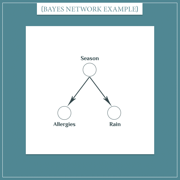
The second situation in which conditional independence arises is when two nodes have a common parent. That is, when they’re siblings:
So, let’s construct its sample space:
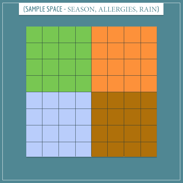
So far, I’ve represented the 4 seasons (associated with the “Seasons” node), which I assumed are equally likely:
- Green: Spring
- Orange: Summer
- Brown: Fall
- Gray: Winter
The second step is to represent the “Allergies” node on the same sample space:
Notice how allergies (the squares colored with pinkish color) are most likely to be triggered during spring and least likely to be triggered during winter (I don’t have much expertise in allergies, but I thought this distribution would be relatively realistic).
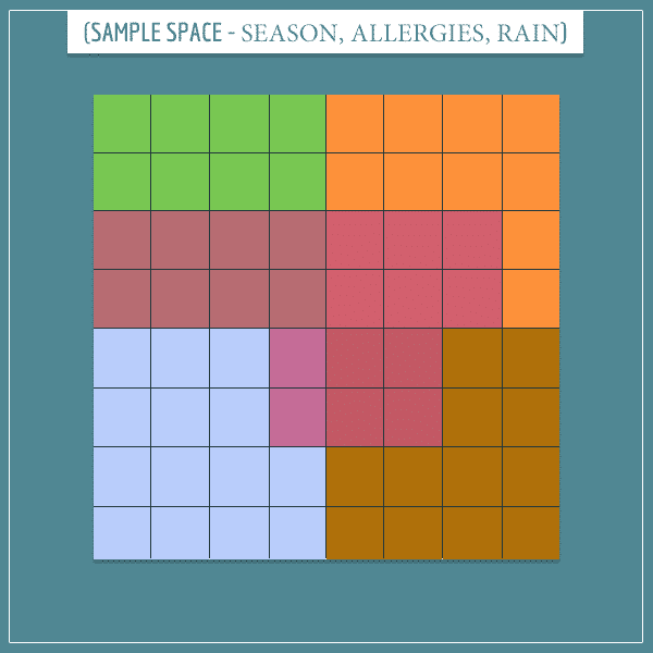
Finally, let’s also add the “Rain” node to the sample space in a way that makes sense:
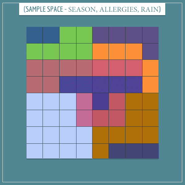
In this case, information about one of the sibling nodes will update the probability of the other, as the parent is a mediating node.
For example, notice that P(Rain | Winter) = 0. This means that if it’s raining, you can exclude winter from the list of possible seasons. Therefore, you’re in one of the other 3 seasons during which allergies are more likely. So, the information that it’s raining indirectly increases P(Allergies).
But what happens when you know the “Season” node’s current state? For the same reason as in the first case, this node can no longer be updated (because its state is known with certainty) and this blocks the information path between the “Allergies” and “Rain” nodes.
Let’s look at an example.
Conditioning on the parent node
Imagine you know the season is definitely fall. This means the top left square of the prior sample space above becomes the posterior sample space:
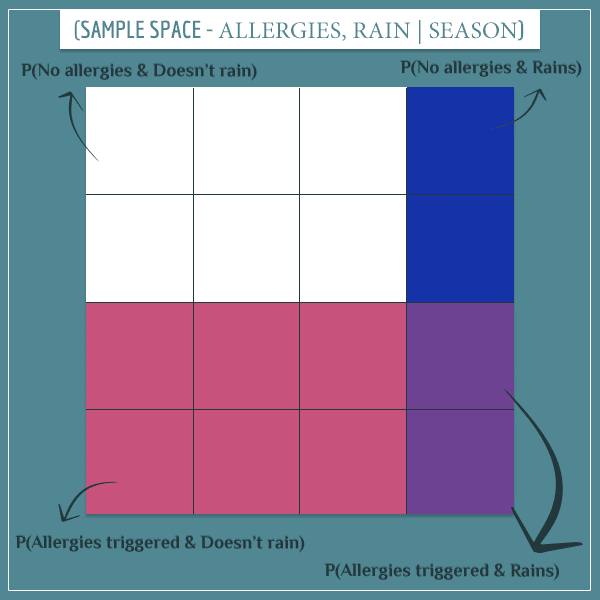
Eight of the “Spring” squares from the prior sample space were dark pink and 4 were dark blue, so the posterior has the same number of each. Therefore:
![\[ P(\textrm{Allergies triggered}) = \frac{8}{16} = \frac{1}{2} \]](https://www.probabilisticworld.com/wp-content/ql-cache/quicklatex.com-64c03dc6a138988f7552416710d81629_l3.png "Rendered by QuickLaTeX.com")
![\[ P(\textrm{Rains}) = \frac{4}{16} = \frac{1}{4} \]](https://www.probabilisticworld.com/wp-content/ql-cache/quicklatex.com-230bf87f3a628bde051405042a68b099_l3.png "Rendered by QuickLaTeX.com")
Notice the same pattern of independence between the events. For example, two of the “Allergies triggered” squares are also “Rains” squares:
![\[ P(\textrm{Rains} \mathbin{\vert} \textrm{Allergies triggered}) = \frac{1}{4} \]](https://www.probabilisticworld.com/wp-content/ql-cache/quicklatex.com-2746641a92feb0562fbb0c0f79fe2752_l3.png "Rendered by QuickLaTeX.com")
And 2 of the “Rains” squares are also “Allergies triggered” squares:
![\[ P(\textrm{Allergies triggered} \mathbin{\vert} \textrm{Rains}) = \frac{2}{4} = \frac{1}{2} \]](https://www.probabilisticworld.com/wp-content/ql-cache/quicklatex.com-c56e1bab47e5c6461a26085db5616130_l3.png "Rendered by QuickLaTeX.com")
Again, we get the same conditional independence result:
![\[ \textrm{Allergies} \perp\!\!\!\perp \textrm{Rain} \mathbin{\vert} \textrm{Season} \]](https://www.probabilisticworld.com/wp-content/ql-cache/quicklatex.com-2b9d0aa14f4f88fd0684a7e1b1119f46_l3.png "Rendered by QuickLaTeX.com")
Or, more specifically:
![\[ P(\textrm{Allergies} \mathbin{\vert} \textrm{Rain}) = P(\textrm{Allergies}) \]](https://www.probabilisticworld.com/wp-content/ql-cache/quicklatex.com-a43515ec8c7cea421c0ca3efe9ec4900_l3.png "Rendered by QuickLaTeX.com")
![\[ P(\textrm{Rain} \mathbin{\vert} \textrm{Allergies}) = P(\textrm{Rain}) \]](https://www.probabilisticworld.com/wp-content/ql-cache/quicklatex.com-bd6c7a8bd6e08e5dfc765d65d94eaaf8_l3.png "Rendered by QuickLaTeX.com")
Conditional dependence
So far, I talked about situations in which two dependent nodes can become independent. But the opposite can also happen.
Consider another part of the large network from the beginning:
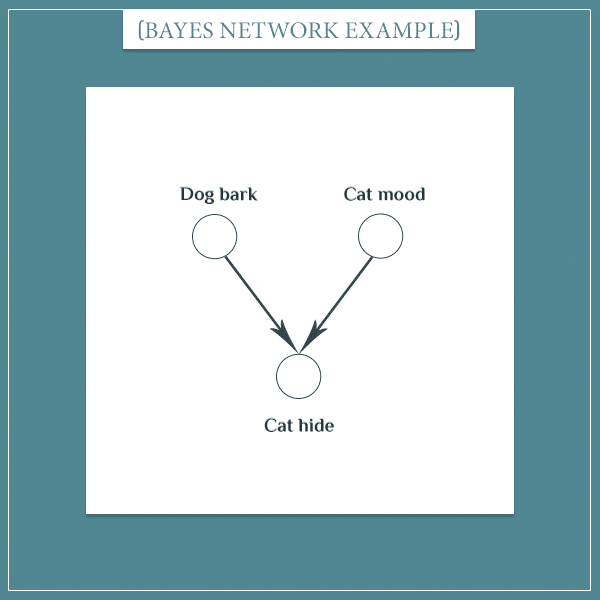
Here I’m assuming that the cat’s mood is independent of the dog’s “decision” to start barking or not. However, the cat’s “decision” to hide is dependent both on the dog’s behavior and on its own current mood (stressed, relaxed, and so on).
Let’s start building the joint sample space of this network. First, let’s represent the “Dog bark” and “Cat mood” nodes:
The gray rectangles represent the “Dog barks” event and the red rectangles represent the “Cat stressed” event.
Maybe by now you’re able to recognize the pattern of independence I’ve been pointing at. As you can see, it’s also present here.
Now, let’s distribute the “Cat hides” event over the current sample space in a relatively sensible way:
Notice how the beige rectangles (representing “Cat hides”) are disproportionately spread over the “Dog barks” and “Cat stressed” rectangles. It’s precisely this disproportionality that will make the parent nodes conditionally dependent, given their child.
Conditioning on the child node
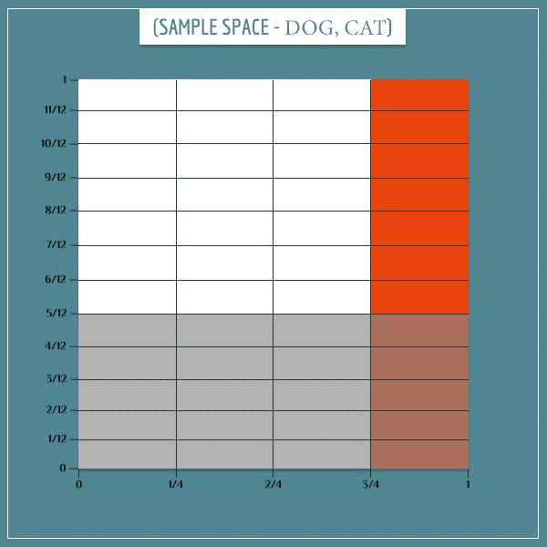
So, what happens if you observe the “Cat hide” node? Let’s say we saw that the cat’s currently under the couch. This means the posterior sample space will consist of the 20 “Cat hides” rectangles only:
The posterior probabilities of the two main events are now:
![\[ P(\textrm{Dog barks}) = \frac{13}{20} \]](https://www.probabilisticworld.com/wp-content/ql-cache/quicklatex.com-040d190bc5ac7decf4b09a7189c10eaf_l3.png "Rendered by QuickLaTeX.com")
![\[ P(\textrm{Cat stressed}) = \frac{8}{20} = \frac{2}{5} \]](https://www.probabilisticworld.com/wp-content/ql-cache/quicklatex.com-1be413a7035105e856c831525e158e65_l3.png "Rendered by QuickLaTeX.com")
And the conditional probabilities:
![\[ P(\textrm{Dog barks} \mathbin{\vert} \textrm{Cat stressed}) = \frac{4}{8} = \frac{1}{2} \]](https://www.probabilisticworld.com/wp-content/ql-cache/quicklatex.com-2c28a45fdbdb52e147e5f7ca4c76b285_l3.png "Rendered by QuickLaTeX.com")
![\[ P(\textrm{Cat stressed} \mathbin{\vert} \textrm{Dog barks}) = \frac{4}{13} \]](https://www.probabilisticworld.com/wp-content/ql-cache/quicklatex.com-2cc00a0dd0e4870fd4814e152ca6e646_l3.png "Rendered by QuickLaTeX.com")
Specifically, notice that:
![\[ P(\textrm{Dog barks} \mathbin{\vert} \textrm{Cat stressed}) \neq P(\textrm{Dog barks}) \]](https://www.probabilisticworld.com/wp-content/ql-cache/quicklatex.com-faad6ad9c3b3ff7c5f399a3c9b1eb75b_l3.png "Rendered by QuickLaTeX.com")
![\[ P(\textrm{Cat stressed} \mathbin{\vert} \textrm{Dog barks}) \neq P(\textrm{Cat stressed}) \]](https://www.probabilisticworld.com/wp-content/ql-cache/quicklatex.com-bc73b357dfb944ec16c60b3e2bc4cd80_l3.png "Rendered by QuickLaTeX.com")
Which means the events are no longer independent!
The intuition behind this is that both parent nodes are potential explanations of the child node, so there’s some competition between them. It’s limited because one event’s occurrence doesn’t exclude the other. It simply makes it less likely.
For example, P(Dog barks | Cat stressed) = 1/2, which is less than P(Dog barks) = 13/20.
This phenomenon is known as explaining away because, generally, the more likely one explanation becomes, the less likely the other explanations will be, and vice versa.
By the way, the most frequently used notation for conditional dependence is very similar to the notation for conditional independence:
Basically, observing a node opens the information flow between its parents and they become dependent. And this is the reason to call this dependence conditional — the nodes are dependent only when one of their children is observed.
The general pattern
In the previous section, I talked about 3 main cases in which the dependence between nodes changes conditionally. Every time a node is observed, it renders its:
- parents independent of its children
- children independent of each other
- parents dependent on each other
However, it’s important to give the full picture of how this works in a general Bayesian network. Let’s go case by case.
Parents conditionally independent on children, given middle nodes
The example I used for this case was this small network:
![]()
Observing the middle node (“Dog bark”) would make its parent (“Rain”) and child (“Cat hide”) independent. But this will happen only if there are no other information paths between the two nodes. Consider the following example:
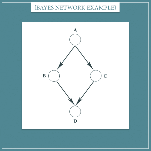
This network is very similar to the previous one. However, instead of a single middle node, there are now 2.
By now, it should be obvious that nodes A and D are not independent. The difference between this case and the simpler case above is that observing one of the 2 middle nodes (B or C) wouldn’t be sufficient to make A and D independent.
For example, observing node B would indeed block one of the paths from A to D. But information can still flow between A and D through node C and, therefore, they’re not conditionally independent, given only node B.
On the other hand, observing both node B and C blocks all paths between A and D. Therefore, the following is true:
- A and D are conditionally independent, given B and C.
In the most general case, two sets of nodes are conditionally independent, given a third set of nodes, if the third set of nodes blocks all information paths between them.
Siblings independent of each other, given parents
I illustrated this second case with the following example:
Here, the sibling nodes “Allergies” and “Rain” were able to influence each other through their common parent “Season”. But if “Season” is in a fixed state, the siblings become independent. Hence, siblings are conditionally independent, given their parents.
Look at the situation in which a pair of siblings have more than one parent node:
In this case, observing one of the parents (A or B) isn’t enough because information can still flow between C and D through the other parent.
This situation is analogous to the previous case and the general idea is the same. Two sets of nodes are conditionally independent, given a third set, if the third set blocks all information paths between them.
Parents conditionally dependent on each other, given their successors
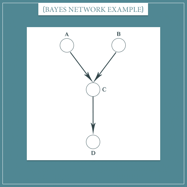
Take a look at the last graph again. I gave it as an example for conditional independence, but it can also be used to illustrate the general concept of conditional dependence.
When nodes C and D are unobserved, nodes A and B are independent. However, if one of the nodes is observed, it opens the information path between A and B and they’re no longer independent.
This should remind you of the simpler configuration from another early example:
In short, if two nodes have one or more children in common, it’s enough to observe either of the children for the nodes to become dependent. Hence, the more general principle can be stated in the following way: two sets of nodes are conditionally dependent, given any of their common children.
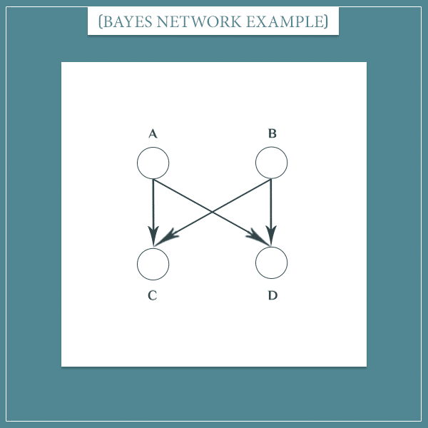
But that’s not the full story. For two nodes to become dependent, you don’t have to necessarily observe the states of their children. Updating the probabilities of any of their children would still render its parents dependent, even if you don’t have full certainty about the child’s state. Take a look at this example:
In this case, if node C is not observed, nodes A and B would be independent. However, observing node D would update the probability distribution of node C, which would partially open the information flow between A and B.
So, in general, two nodes are independent only if none of their common successor nodes are observed.
D-separation
The concept of d-separation summarizes the three general cases I described in this section. Basically, two sets of nodes are said to be d-separated from each other if there are no open information paths between them. Them being d-separated is just another way of saying that they are independent.
Open information paths consist of unobserved common middle or parent nodes, as well as observed common successor nodes.
D-separation is very useful because it allows you to drop non-existent dependencies from the posterior distribution. And this can greatly simplify the final expression.
Summary
As I said in the beginning, this post is an informal Part 3, after Part 1 and Part 2, of the Bayesian belief networks series.
I showed how the dependence between nodes can be conditional on certain other nodes. The three general cases are:
- Parents and children of middle nodes are conditionally independent, given all the middle nodes.
- Sibling nodes are conditionally independent, given all their common parents.
- Parent nodes are conditionally dependent, given any of their common successors (common children, grandchildren, and so on).
If you found this post difficult to follow, try reading the 2 Bayesian network posts I linked to in the beginning. But overall, I hope you found my explanations and examples here useful.
In some of the next few posts, I plan to show a few real-world applications of Bayesian networks in which I’ll also make use of the conditional dependence/independence properties of the graphs. This should give you even better intuition about their usefulness.
Thank you very much. So good. The article is awesome.
It is a very well-written article. I have now gained a better understanding of what d-separation and conditional (in)dependence are. Thank you very much.
Super helpful read, thank you. I hope to read more from you.
This s pretty concise. I read your series for Bayes and the way you break down is fabulous. But I cant find the post of real-world application of Bayes last part you mention in this post
Hi NGhi, and thank you for your feedback! Indeed, as you have noticed, I haven’t had as much time to spend on writing new posts as I wanted. But I’m doing my best to make that change and increase my post frequency significantly in 2020.
In fact, one of my very next posts is going to be a very interesting real world application of Bayes’ theorem and Bayesian networks. I am going to leave the topic as a surprise for now, but I will link to that post here as well once it’s ready. Of course, feel free to subscribe to my mail list to get an instant notification the moment it is published.
Cheers
Hi,
Just to make things clear, the last example where there are four nodes: A, B, C, and D, where node A and B are parents of node C and node D is child succesor of node C.
If node C is observed, then node A and B are dependent; the same thing happened if node D is observed:
if node D is observed, then node A and B are dependent
Hi, Ridzky. Yes, you are correct. In that example, nodes A and B are conditionally dependent, given C or D (or both). Of course, node C is what’s causing the conditional dependence and if it’s already observed, then D is irrelevant. In other words, as far as conditional dependence of A and B goes, observing D only matters if C isn’t already observed.
Thanks, the overall ideas were helpful, but not far into it the colored pictures became very confusing, starting with “The new sample space consists only of the 27 gray rectangles corresponding to the “Dog barks” event.” in which the squares are not colored the same as in the preceding picture from which the squares in this one were obtained. For example there are 2 light blue cells in the preceding and 3 in the following picture. I don’t want to have to construct and remember a color translation table. After trying to figure that one out for a while I just ignored further pictures. The text made sense without them. (Separately, I might suggest cross-hatching as a more decipherable way of multiply labeling cells, than blending colors.)
That is, I ignored colored cell pictures. The graphs were still useful.